paper

*The author of this computation has been verified*

R Software Module: /rwasp_centraltendency.wasp (opens new window with default values)

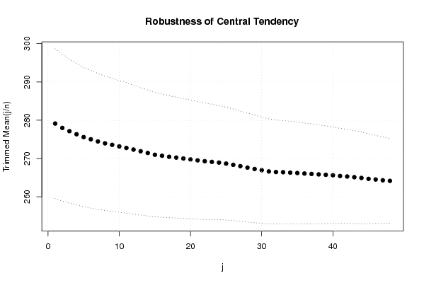
Title produced by software: Central Tendency

Date of computation: Fri, 20 Nov 2009 04:21:53 -0700

Cite this page as follows:

Statistical Computations at FreeStatistics.org, Office for Research Development and Education, URL http://www.freestatistics.org/blog/date/2009/Nov/20/t1258716201l93up138w5pgqgw.htm/, Retrieved Fri, 20 Nov 2009 12:23:23 +0100

BibTeX entries for LaTeX users:

@Manual{KEY, author = {{YOUR NAME}}, publisher = {Office for Research Development and Education}, title = {Statistical Computations at FreeStatistics.org, URL http://www.freestatistics.org/blog/date/2009/Nov/20/t1258716201l93up138w5pgqgw.htm/}, year = {2009}, } @Manual{R, title = {R: A Language and Environment for Statistical Computing}, author = {{R Development Core Team}}, organization = {R Foundation for Statistical Computing}, address = {Vienna, Austria}, year = {2009}, note = {{ISBN} 3-900051-07-0}, url = {http://www.R-project.org}, }

Original text written by user:

IsPrivate?

No (this computation is public)

User-defined keywords:

Dataseries X:

» Textbox « » Textfile « » CSV «

112 118 132 129 121 135 148 148 136 119 104 118 115 126 141 135 125 149 170 170 158 133 114 140 145 150 178 163 172 178 199 199 184 162 146 166 171 180 193 181 183 218 230 242 209 191 172 194 196 196 236 235 229 243 264 272 237 211 180 201 204 188 235 227 234 264 302 293 259 229 203 229 242 233 267 269 270 315 364 347 312 274 237 278 284 277 317 313 318 374 413 405 355 306 271 306 315 301 356 348 355 422 465 467 404 347 305 336 340 318 362 348 363 435 491 505 404 359 310 337 360 342 406 396 420 472 548 559 463 407 362 405 417 391 419 461 472 535 622 606 508 461 390 432

Output produced by software:

Summary of computational transaction Raw Input view raw input (R code) Raw Output view raw output of R engine Computing time 1 seconds R Server 'Gwilym Jenkins' @ 72.249.127.135 Central Tendency - Ungrouped Data Measure Value S.E. Value/S.E. Arithmetic Mean 280.298611111111 9.9971930785786 28.0377310819092 Geometric Mean 255.232771586034 Harmonic Mean 231.659113395685 Quadratic Mean 304.728214516185 Winsorized Mean ( 1 / 48 ) 280.243055555556 9.96450697402584 28.1241265911154 Winsorized Mean ( 2 / 48 ) 279.618055555556 9.82161700036816 28.4696558158472 Winsorized Mean ( 3 / 48 ) 279.409722222222 9.77435005099722 28.5860155165730 Winsorized Mean ( 4 / 48 ) 279.131944444444 9.6965880387294 28.7866147689843 Winsorized Mean ( 5 / 48 ) 278.194444444444 9.53099000990649 29.1884100345599 Winsorized Mean ( 6 / 48 ) 278.111111111111 9.50513147669147 29.2590493664497 Winsorized Mean ( 7 / 48 ) 277.527777777778 9.3828137313047 29.5783104861005 Winsorized Mean ( 8 / 48 ) 276.694444444444 9.19460817653402 30.093119699283 Winsorized Mean ( 9 / 48 ) 276.756944444444 9.18741689636644 30.1234773131825 Winsorized Mean ( 10 / 48 ) 276.618055555556 9.11249620440785 30.3559035143138 Winsorized Mean ( 11 / 48 ) 276.694444444444 9.06446671866159 30.5251762770331 Winsorized Mean ( 12 / 48 ) 276.611111111111 9.03104865735461 30.6289027560324 Winsorized Mean ( 13 / 48 ) 276.611111111111 8.98507412452583 30.7856237219088 Winsorized Mean ( 14 / 48 ) 276.611111111111 8.98507412452583 30.7856237219088 Winsorized Mean ( 15 / 48 ) 274.006944444444 8.60154334040167 31.8555558695411 Winsorized Mean ( 16 / 48 ) 274.118055555556 8.50867111379589 32.2163181405734 Winsorized Mean ( 17 / 48 ) 273.055555555556 8.34533970616904 32.7195255279671 Winsorized Mean ( 18 / 48 ) 273.305555555556 8.25938799619298 33.0902913970782 Winsorized Mean ( 19 / 48 ) 273.305555555556 8.22872145694721 33.2136112499972 Winsorized Mean ( 20 / 48 ) 273.305555555556 8.16449758179813 33.4748773966032 Winsorized Mean ( 21 / 48 ) 272.722222222222 8.09324569732642 33.6975093085726 Winsorized Mean ( 22 / 48 ) 271.958333333333 7.96687778904112 34.1361246569424 Winsorized Mean ( 23 / 48 ) 271.958333333333 7.93076511166547 34.2915632355958 Winsorized Mean ( 24 / 48 ) 273.125 7.77023435045024 35.1501624895231 Winsorized Mean ( 25 / 48 ) 273.819444444444 7.69898966101939 35.5656334792622 Winsorized Mean ( 26 / 48 ) 273.819444444444 7.65919908928945 35.7504017394392 Winsorized Mean ( 27 / 48 ) 274.381944444444 7.60270264207722 36.0900534141472 Winsorized Mean ( 28 / 48 ) 273.604166666667 7.34211713525314 37.2650233749279 Winsorized Mean ( 29 / 48 ) 272.597222222222 7.22572376043573 37.7259401632292 Winsorized Mean ( 30 / 48 ) 272.597222222222 7.18122957585258 37.9596863382352 Winsorized Mean ( 31 / 48 ) 269.368055555556 6.7766047862394 39.7497071250983 Winsorized Mean ( 32 / 48 ) 267.145833333333 6.54150404197069 40.8385948582022 Winsorized Mean ( 33 / 48 ) 268.291666666667 6.37975164568387 42.0536223926797 Winsorized Mean ( 34 / 48 ) 268.055555555556 6.35529239542982 42.1783198753087 Winsorized Mean ( 35 / 48 ) 268.541666666667 6.30734666020482 42.5760119324005 Winsorized Mean ( 36 / 48 ) 268.041666666667 6.25574231156358 42.8472998593945 Winsorized Mean ( 37 / 48 ) 268.041666666667 6.20411575894803 43.2038467818846 Winsorized Mean ( 38 / 48 ) 267.777777777778 6.0716506945483 44.1029616572334 Winsorized Mean ( 39 / 48 ) 267.777777777778 6.01775930102673 44.4979209673758 Winsorized Mean ( 40 / 48 ) 268.888888888889 5.91049623345049 45.4934540634864 Winsorized Mean ( 41 / 48 ) 267.75 5.62793996380632 47.575134369222 Winsorized Mean ( 42 / 48 ) 268.333333333333 5.57255073357988 48.1526945490817 Winsorized Mean ( 43 / 48 ) 268.333333333333 5.5145407138908 48.6592351485261 Winsorized Mean ( 44 / 48 ) 268.944444444444 5.45717574139167 49.2827164066846 Winsorized Mean ( 45 / 48 ) 267.381944444444 5.30212859617042 50.4291700200495 Winsorized Mean ( 46 / 48 ) 267.701388888889 5.14950416534481 51.985857335638 Winsorized Mean ( 47 / 48 ) 266.722222222222 5.05382301656813 52.776328206947 Winsorized Mean ( 48 / 48 ) 267.055555555556 4.95912564214639 53.851338890452 Trimmed Mean ( 1 / 48 ) 279.133802816901 9.76706648594188 28.5790829025961 Trimmed Mean ( 2 / 48 ) 277.992857142857 9.55067888994526 29.1071305345133 Trimmed Mean ( 3 / 48 ) 277.144927536232 9.39595037768446 29.4962102178036 Trimmed Mean ( 4 / 48 ) 276.345588235294 9.24536849648412 29.8901648258135 Trimmed Mean ( 5 / 48 ) 275.597014925373 9.10451366971599 30.2703719191593 Trimmed Mean ( 6 / 48 ) 275.030303030303 8.9928065129399 30.58336712066 Trimmed Mean ( 7 / 48 ) 274.461538461538 8.87580884030334 30.9224255952045 Trimmed Mean ( 8 / 48 ) 273.96875 8.7713107857995 31.2346417417506 Trimmed Mean ( 9 / 48 ) 273.579365079365 8.6895036347882 31.4838886750789 Trimmed Mean ( 10 / 48 ) 273.169354838710 8.60012778842319 31.7634064933813 Trimmed Mean ( 11 / 48 ) 272.762295081967 8.51250944996314 32.0425247907535 Trimmed Mean ( 12 / 48 ) 272.333333333333 8.42209589985802 32.3355773398311 Trimmed Mean ( 13 / 48 ) 271.898305084746 8.3262237367141 32.6556568358622 Trimmed Mean ( 14 / 48 ) 271.448275862069 8.22559854894425 33.0004283879024 Trimmed Mean ( 15 / 48 ) 270.982456140351 8.11354929163366 33.3987563765437 Trimmed Mean ( 16 / 48 ) 270.723214285714 8.03631767897612 33.6874704435783 Trimmed Mean ( 17 / 48 ) 270.445454545455 7.96039598978601 33.9738695025302 Trimmed Mean ( 18 / 48 ) 270.240740740741 7.89365399178675 34.2351895613771 Trimmed Mean ( 19 / 48 ) 270.009433962264 7.82750346362996 34.4949619271135 Trimmed Mean ( 20 / 48 ) 269.769230769231 7.75578551028098 34.7829669105247 Trimmed Mean ( 21 / 48 ) 269.519607843137 7.68128134927983 35.0878447992803 Trimmed Mean ( 22 / 48 ) 269.3 7.60436477533552 35.4138718954494 Trimmed Mean ( 23 / 48 ) 269.122448979592 7.53031974102612 35.7385155258919 Trimmed Mean ( 24 / 48 ) 268.9375 7.44950564267022 36.1013888572076 Trimmed Mean ( 25 / 48 ) 268.670212765957 7.37349480233507 36.4372960134011 Trimmed Mean ( 26 / 48 ) 268.347826086957 7.29321453194246 36.7941769588239 Trimmed Mean ( 27 / 48 ) 268.011111111111 7.20491049161063 37.1983956529623 Trimmed Mean ( 28 / 48 ) 267.625 7.10876672805764 37.6471771036893 Trimmed Mean ( 29 / 48 ) 267.267441860465 7.02614668129215 38.0389784022148 Trimmed Mean ( 30 / 48 ) 266.952380952381 6.94304971924255 38.4488649436755 Trimmed Mean ( 31 / 48 ) 266.621951219512 6.85083554609109 38.9181654450368 Trimmed Mean ( 32 / 48 ) 266.4625 6.78850815414261 39.251996749447 Trimmed Mean ( 33 / 48 ) 266.423076923077 6.73968963137491 39.5304667566311 Trimmed Mean ( 34 / 48 ) 266.315789473684 6.69729483294629 39.7646805339352 Trimmed Mean ( 35 / 48 ) 266.216216216216 6.64750248230333 40.047554239344 Trimmed Mean ( 36 / 48 ) 266.083333333333 6.59144030463107 40.3680107891422 Trimmed Mean ( 37 / 48 ) 265.971428571429 6.52864278200131 40.7391608719472 Trimmed Mean ( 38 / 48 ) 265.852941176471 6.45771226673023 41.1682853301052 Trimmed Mean ( 39 / 48 ) 265.742424242424 6.38695168274328 41.6070822894161 Trimmed Mean ( 40 / 48 ) 265.625 6.30635308920411 42.1202232483184 Trimmed Mean ( 41 / 48 ) 265.435483870968 6.22037647868813 42.6719322826177 Trimmed Mean ( 42 / 48 ) 265.3 6.15199659841361 43.1242111005737 Trimmed Mean ( 43 / 48 ) 265.120689655172 6.07251389763974 43.6591326300989 Trimmed Mean ( 44 / 48 ) 264.928571428571 5.98009996131418 44.3016961492983 Trimmed Mean ( 45 / 48 ) 264.685185185185 5.87119037010693 45.0820308148796 Trimmed Mean ( 46 / 48 ) 264.519230769231 5.7590829555713 45.9307901639681 Trimmed Mean ( 47 / 48 ) 264.32 5.64120699199476 46.8552209438666 Trimmed Mean ( 48 / 48 ) 264.166666666667 5.50695348110241 47.9696564667156 Median 265.5 Midrange 363 Midmean - Weighted Average at Xnp 264.904109589041 Midmean - Weighted Average at X(n+1)p 264.904109589041 Midmean - Empirical Distribution Function 264.904109589041 Midmean - Empirical Distribution Function - Averaging 264.904109589041 Midmean - Empirical Distribution Function - Interpolation 264.904109589041 Midmean - Closest Observation 264.904109589041 Midmean - True Basic - Statistics Graphics Toolkit 264.904109589041 Midmean - MS Excel (old versions) 267.493333333333 Number of observations 144

Charts produced by software:

http://www.freestatistics.org/blog/date/2009/Nov/20/t1258716201l93up138w5pgqgw/1xba51258716111.png (open in new window) http://www.freestatistics.org/blog/date/2009/Nov/20/t1258716201l93up138w5pgqgw/1xba51258716111.ps (open in new window) http://www.freestatistics.org/blog/date/2009/Nov/20/t1258716201l93up138w5pgqgw/2pnw51258716111.png (open in new window) http://www.freestatistics.org/blog/date/2009/Nov/20/t1258716201l93up138w5pgqgw/2pnw51258716111.ps (open in new window)

Parameters (Session):

Parameters (R input):

R code (references can be found in the software module):

geomean <- function(x) { return(exp(mean(log(x)))) } harmean <- function(x) { return(1/mean(1/x)) } quamean <- function(x) { return(sqrt(mean(x*x))) } winmean <- function(x) { x <-sort(x[!is.na(x)]) n<-length(x) denom <- 3 nodenom <- n/denom if (nodenom>40) denom <- n/40 sqrtn = sqrt(n) roundnodenom = floor(nodenom) win <- array(NA,dim=c(roundnodenom,2)) for (j in 1:roundnodenom) { win[j,1] <- (j*x[j+1]+sum(x[(j+1):(n-j)])+j*x[n-j])/n win[j,2] <- sd(c(rep(x[j+1],j),x[(j+1):(n-j)],rep(x[n-j],j)))/sqrtn } return(win) } trimean <- function(x) { x <-sort(x[!is.na(x)]) n<-length(x) denom <- 3 nodenom <- n/denom if (nodenom>40) denom <- n/40 sqrtn = sqrt(n) roundnodenom = floor(nodenom) tri <- array(NA,dim=c(roundnodenom,2)) for (j in 1:roundnodenom) { tri[j,1] <- mean(x,trim=j/n) tri[j,2] <- sd(x[(j+1):(n-j)]) / sqrt(n-j*2) } return(tri) } midrange <- function(x) { return((max(x)+min(x))/2) } q1 <- function(data,n,p,i,f) { np <- n*p; i <<- floor(np) f <<- np - i qvalue <- (1-f)*data[i] + f*data[i+1] } q2 <- function(data,n,p,i,f) { np <- (n+1)*p i <<- floor(np) f <<- np - i qvalue <- (1-f)*data[i] + f*data[i+1] } q3 <- function(data,n,p,i,f) { np <- n*p i <<- floor(np) f <<- np - i if (f==0) { qvalue <- data[i] } else { qvalue <- data[i+1] } } q4 <- function(data,n,p,i,f) { np <- n*p i <<- floor(np) f <<- np - i if (f==0) { qvalue <- (data[i]+data[i+1])/2 } else { qvalue <- data[i+1] } } q5 <- function(data,n,p,i,f) { np <- (n-1)*p i <<- floor(np) f <<- np - i if (f==0) { qvalue <- data[i+1] } else { qvalue <- data[i+1] + f*(data[i+2]-data[i+1]) } } q6 <- function(data,n,p,i,f) { np <- n*p+0.5 i <<- floor(np) f <<- np - i qvalue <- data[i] } q7 <- function(data,n,p,i,f) { np <- (n+1)*p i <<- floor(np) f <<- np - i if (f==0) { qvalue <- data[i] } else { qvalue <- f*data[i] + (1-f)*data[i+1] } } q8 <- function(data,n,p,i,f) { np <- (n+1)*p i <<- floor(np) f <<- np - i if (f==0) { qvalue <- data[i] } else { if (f == 0.5) { qvalue <- (data[i]+data[i+1])/2 } else { if (f < 0.5) { qvalue <- data[i] } else { qvalue <- data[i+1] } } } } midmean <- function(x,def) { x <-sort(x[!is.na(x)]) n<-length(x) if (def==1) { qvalue1 <- q1(x,n,0.25,i,f) qvalue3 <- q1(x,n,0.75,i,f) } if (def==2) { qvalue1 <- q2(x,n,0.25,i,f) qvalue3 <- q2(x,n,0.75,i,f) } if (def==3) { qvalue1 <- q3(x,n,0.25,i,f) qvalue3 <- q3(x,n,0.75,i,f) } if (def==4) { qvalue1 <- q4(x,n,0.25,i,f) qvalue3 <- q4(x,n,0.75,i,f) } if (def==5) { qvalue1 <- q5(x,n,0.25,i,f) qvalue3 <- q5(x,n,0.75,i,f) } if (def==6) { qvalue1 <- q6(x,n,0.25,i,f) qvalue3 <- q6(x,n,0.75,i,f) } if (def==7) { qvalue1 <- q7(x,n,0.25,i,f) qvalue3 <- q7(x,n,0.75,i,f) } if (def==8) { qvalue1 <- q8(x,n,0.25,i,f) qvalue3 <- q8(x,n,0.75,i,f) } midm <- 0 myn <- 0 roundno4 <- round(n/4) round3no4 <- round(3*n/4) for (i in 1:n) { if ((x[i]>=qvalue1) & (x[i]<=qvalue3)){ midm = midm + x[i] myn = myn + 1 } } midm = midm / myn return(midm) } (arm <- mean(x)) sqrtn <- sqrt(length(x)) (armse <- sd(x) / sqrtn) (armose <- arm / armse) (geo <- geomean(x)) (har <- harmean(x)) (qua <- quamean(x)) (win <- winmean(x)) (tri <- trimean(x)) (midr <- midrange(x)) midm <- array(NA,dim=8) for (j in 1:8) midm[j] <- midmean(x,j) midm bitmap(file='test1.png') lb <- win[,1] - 2*win[,2] ub <- win[,1] + 2*win[,2] if ((ylimmin == '') | (ylimmax == '')) plot(win[,1],type='b',main=main, xlab='j', pch=19, ylab='Winsorized Mean(j/n)', ylim=c(min(lb),max(ub))) else plot(win[,1],type='l',main=main, xlab='j', pch=19, ylab='Winsorized Mean(j/n)', ylim=c(ylimmin,ylimmax)) lines(ub,lty=3) lines(lb,lty=3) grid() dev.off() bitmap(file='test2.png') lb <- tri[,1] - 2*tri[,2] ub <- tri[,1] + 2*tri[,2] if ((ylimmin == '') | (ylimmax == '')) plot(tri[,1],type='b',main=main, xlab='j', pch=19, ylab='Trimmed Mean(j/n)', ylim=c(min(lb),max(ub))) else plot(tri[,1],type='l',main=main, xlab='j', pch=19, ylab='Trimmed Mean(j/n)', ylim=c(ylimmin,ylimmax)) lines(ub,lty=3) lines(lb,lty=3) grid() dev.off() load(file='createtable') a<-table.start() a<-table.row.start(a) a<-table.element(a,'Central Tendency - Ungrouped Data',4,TRUE) a<-table.row.end(a) a<-table.row.start(a) a<-table.element(a,'Measure',header=TRUE) a<-table.element(a,'Value',header=TRUE) a<-table.element(a,'S.E.',header=TRUE) a<-table.element(a,'Value/S.E.',header=TRUE) a<-table.row.end(a) a<-table.row.start(a) a<-table.element(a,hyperlink('http://www.xycoon.com/arithmetic_mean.htm', 'Arithmetic Mean', 'click to view the definition of the Arithmetic Mean'),header=TRUE) a<-table.element(a,arm) a<-table.element(a,hyperlink('http://www.xycoon.com/arithmetic_mean_standard_error.htm', armse, 'click to view the definition of the Standard Error of the Arithmetic Mean')) a<-table.element(a,armose) a<-table.row.end(a) a<-table.row.start(a) a<-table.element(a,hyperlink('http://www.xycoon.com/geometric_mean.htm', 'Geometric Mean', 'click to view the definition of the Geometric Mean'),header=TRUE) a<-table.element(a,geo) a<-table.element(a,'') a<-table.element(a,'') a<-table.row.end(a) a<-table.row.start(a) a<-table.element(a,hyperlink('http://www.xycoon.com/harmonic_mean.htm', 'Harmonic Mean', 'click to view the definition of the Harmonic Mean'),header=TRUE) a<-table.element(a,har) a<-table.element(a,'') a<-table.element(a,'') a<-table.row.end(a) a<-table.row.start(a) a<-table.element(a,hyperlink('http://www.xycoon.com/quadratic_mean.htm', 'Quadratic Mean', 'click to view the definition of the Quadratic Mean'),header=TRUE) a<-table.element(a,qua) a<-table.element(a,'') a<-table.element(a,'') a<-table.row.end(a) for (j in 1:length(win[,1])) { a<-table.row.start(a) mylabel <- paste('Winsorized Mean (',j) mylabel <- paste(mylabel,'/') mylabel <- paste(mylabel,length(win[,1])) mylabel <- paste(mylabel,')') a<-table.element(a,hyperlink('http://www.xycoon.com/winsorized_mean.htm', mylabel, 'click to view the definition of the Winsorized Mean'),header=TRUE) a<-table.element(a,win[j,1]) a<-table.element(a,win[j,2]) a<-table.element(a,win[j,1]/win[j,2]) a<-table.row.end(a) } for (j in 1:length(tri[,1])) { a<-table.row.start(a) mylabel <- paste('Trimmed Mean (',j) mylabel <- paste(mylabel,'/') mylabel <- paste(mylabel,length(tri[,1])) mylabel <- paste(mylabel,')') a<-table.element(a,hyperlink('http://www.xycoon.com/arithmetic_mean.htm', mylabel, 'click to view the definition of the Trimmed Mean'),header=TRUE) a<-table.element(a,tri[j,1]) a<-table.element(a,tri[j,2]) a<-table.element(a,tri[j,1]/tri[j,2]) a<-table.row.end(a) } a<-table.row.start(a) a<-table.element(a,hyperlink('http://www.xycoon.com/median_1.htm', 'Median', 'click to view the definition of the Median'),header=TRUE) a<-table.element(a,median(x)) a<-table.element(a,'') a<-table.element(a,'') a<-table.row.end(a) a<-table.row.start(a) a<-table.element(a,hyperlink('http://www.xycoon.com/midrange.htm', 'Midrange', 'click to view the definition of the Midrange'),header=TRUE) a<-table.element(a,midr) a<-table.element(a,'') a<-table.element(a,'') a<-table.row.end(a) a<-table.row.start(a) mymid <- hyperlink('http://www.xycoon.com/midmean.htm', 'Midmean', 'click to view the definition of the Midmean') mylabel <- paste(mymid,hyperlink('http://www.xycoon.com/method_1.htm','Weighted Average at Xnp',''),sep=' - ') a<-table.element(a,mylabel,header=TRUE) a<-table.element(a,midm[1]) a<-table.element(a,'') a<-table.element(a,'') a<-table.row.end(a) a<-table.row.start(a) mymid <- hyperlink('http://www.xycoon.com/midmean.htm', 'Midmean', 'click to view the definition of the Midmean') mylabel <- paste(mymid,hyperlink('http://www.xycoon.com/method_2.htm','Weighted Average at X(n+1)p',''),sep=' - ') a<-table.element(a,mylabel,header=TRUE) a<-table.element(a,midm[2]) a<-table.element(a,'') a<-table.element(a,'') a<-table.row.end(a) a<-table.row.start(a) mymid <- hyperlink('http://www.xycoon.com/midmean.htm', 'Midmean', 'click to view the definition of the Midmean') mylabel <- paste(mymid,hyperlink('http://www.xycoon.com/method_3.htm','Empirical Distribution Function',''),sep=' - ') a<-table.element(a,mylabel,header=TRUE) a<-table.element(a,midm[3]) a<-table.element(a,'') a<-table.element(a,'') a<-table.row.end(a) a<-table.row.start(a) mymid <- hyperlink('http://www.xycoon.com/midmean.htm', 'Midmean', 'click to view the definition of the Midmean') mylabel <- paste(mymid,hyperlink('http://www.xycoon.com/method_4.htm','Empirical Distribution Function - Averaging',''),sep=' - ') a<-table.element(a,mylabel,header=TRUE) a<-table.element(a,midm[4]) a<-table.element(a,'') a<-table.element(a,'') a<-table.row.end(a) a<-table.row.start(a) mymid <- hyperlink('http://www.xycoon.com/midmean.htm', 'Midmean', 'click to view the definition of the Midmean') mylabel <- paste(mymid,hyperlink('http://www.xycoon.com/method_5.htm','Empirical Distribution Function - Interpolation',''),sep=' - ') a<-table.element(a,mylabel,header=TRUE) a<-table.element(a,midm[5]) a<-table.element(a,'') a<-table.element(a,'') a<-table.row.end(a) a<-table.row.start(a) mymid <- hyperlink('http://www.xycoon.com/midmean.htm', 'Midmean', 'click to view the definition of the Midmean') mylabel <- paste(mymid,hyperlink('http://www.xycoon.com/method_6.htm','Closest Observation',''),sep=' - ') a<-table.element(a,mylabel,header=TRUE) a<-table.element(a,midm[6]) a<-table.element(a,'') a<-table.element(a,'') a<-table.row.end(a) a<-table.row.start(a) mymid <- hyperlink('http://www.xycoon.com/midmean.htm', 'Midmean', 'click to view the definition of the Midmean') mylabel <- paste(mymid,hyperlink('http://www.xycoon.com/method_7.htm','True Basic - Statistics Graphics Toolkit',''),sep=' - ') a<-table.element(a,mylabel,header=TRUE) a<-table.element(a,midm[7]) a<-table.element(a,'') a<-table.element(a,'') a<-table.row.end(a) a<-table.row.start(a) mymid <- hyperlink('http://www.xycoon.com/midmean.htm', 'Midmean', 'click to view the definition of the Midmean') mylabel <- paste(mymid,hyperlink('http://www.xycoon.com/method_8.htm','MS Excel (old versions)',''),sep=' - ') a<-table.element(a,mylabel,header=TRUE) a<-table.element(a,midm[8]) a<-table.element(a,'') a<-table.element(a,'') a<-table.row.end(a) a<-table.row.start(a) a<-table.element(a,'Number of observations',header=TRUE) a<-table.element(a,length(x)) a<-table.element(a,'') a<-table.element(a,'') a<-table.row.end(a) a<-table.end(a) table.save(a,file='mytable.tab')

Copyright

This work is licensed under a Creative Commons Attribution-Noncommercial-Share Alike 3.0 License.

Software written by Ed van Stee & Patrick Wessa

Disclaimer

Information provided on this web site is provided "AS IS" without warranty of any kind, either express or implied, including, without limitation, warranties of merchantability, fitness for a particular purpose, and noninfringement. We use reasonable efforts to include accurate and timely information and periodically update the information, and software without notice. However, we make no warranties or representations as to the accuracy or completeness of such information (or software), and we assume no liability or responsibility for errors or omissions in the content of this web site, or any software bugs in online applications. Your use of this web site is AT YOUR OWN RISK. Under no circumstances and under no legal theory shall we be liable to you or any other person for any direct, indirect, special, incidental, exemplary, or consequential damages arising from your access to, or use of, this web site.

Privacy Policy

We may request personal information to be submitted to our servers in order to be able to:

• personalize online software applications according to your needs
• enforce strict security rules with respect to the data that you upload (e.g. statistical data)
• manage user sessions of online applications
• alert you about important changes or upgrades in resources or applications

We NEVER allow other companies to directly offer registered users information about their products and services. Banner references and hyperlinks of third parties NEVER contain any personal data of the visitor.

We do NOT sell, nor transmit by any means, personal information, nor statistical data series uploaded by you to third parties.

We carefully protect your data from loss, misuse, alteration, and destruction. However, at any time, and under any circumstance you are solely responsible for managing your passwords, and keeping them secret.

We store a unique ANONYMOUS USER ID in the form of a small 'Cookie' on your computer. This allows us to track your progress when using this website which is necessary to create state-dependent features. The cookie is used for NO OTHER PURPOSE. At any time you may opt to disallow cookies from this website - this will not affect other features of this website.

We examine cookies that are used by third-parties (banner and online ads) very closely: abuse from third-parties automatically results in termination of the advertising contract without refund. We have very good reason to believe that the cookies that are produced by third parties (banner ads) do NOT cause any privacy or security risk.

FreeStatistics.org is safe. There is no need to download any software to use the applications and services contained in this website. Hence, your system's security is not compromised by their use, and your personal data - other than data you submit in the account application form, and the user-agent information that is transmitted by your browser - is never transmitted to our servers.

As a general rule, we do not log on-line behavior of individuals (other than normal logging of webserver 'hits'). However, in cases of abuse, hacking, unauthorized access, Denial of Service attacks, illegal copying, hotlinking, non-compliance with international webstandards (such as robots.txt), or any other harmful behavior, our system engineers are empowered to log, track, identify, publish, and ban misbehaving individuals - even if this leads to ban entire blocks of IP addresses, or disclosing user's identity.

FreeStatistics.org is powered by