*The author of this computation has been verified*

R Software Module: /rwasp_multipleregression.wasp (opens new window with default values)

Title produced by software: Multiple Regression

Date of computation: Fri, 20 Nov 2009 07:13:54 -0700

Cite this page as follows:

Statistical Computations at FreeStatistics.org, Office for Research Development and Education, URL http://www.freestatistics.org/blog/date/2009/Nov/20/t12587265297a5irk5g86rbmxa.htm/, Retrieved Fri, 20 Nov 2009 15:15:42 +0100

BibTeX entries for LaTeX users:

@Manual{KEY, author = {{YOUR NAME}}, publisher = {Office for Research Development and Education}, title = {Statistical Computations at FreeStatistics.org, URL http://www.freestatistics.org/blog/date/2009/Nov/20/t12587265297a5irk5g86rbmxa.htm/}, year = {2009}, } @Manual{R, title = {R: A Language and Environment for Statistical Computing}, author = {{R Development Core Team}}, organization = {R Foundation for Statistical Computing}, address = {Vienna, Austria}, year = {2009}, note = {{ISBN} 3-900051-07-0}, url = {http://www.R-project.org}, }

Original text written by user:

IsPrivate?

No (this computation is public)

User-defined keywords:

shwws7

Dataseries X:

» Textbox « » Textfile « » CSV «

6539 2605 6699 2682 6962 2755 6981 2760 7024 2735 6940 2659 6774 2654 6671 2670 6965 2785 6969 2845 6822 2723 6878 2746 6691 2767 6837 2940 7018 2977 7167 2993 7076 2892 7171 2824 7093 2771 6971 2686 7142 2738 7047 2723 6999 2731 6650 2632 6475 2606 6437 2605 6639 2646 6422 2627 6272 2535 6232 2456 6003 2404 5673 2319 6050 2519 5977 2504 5796 2382 5752 2394 5609 2381 5839 2501 6069 2532 6006 2515 5809 2429 5797 2389 5502 2261 5568 2272 5864 2439 5764 2373 5615 2327 5615 2364 5681 2388 5915 2553 6334 2663 6494 2694 6620 2679 6578 2611 6495 2580 6538 2627 6737 2732 6651 2707 6530 2633 6563 2683

Output produced by software:

Enter (or paste) a matrix (table) containing all data (time) series. Every column represents a different variable and must be delimited by a space or Tab. Every row represents a period in time (or category) and must be delimited by hard returns. The easiest way to enter data is to copy and paste a block of spreadsheet cells. Please, do not use commas or spaces to seperate groups of digits! Summary of computational transaction Raw Input view raw input (R code) Raw Output view raw output of R engine Computing time 3 seconds R Server 'Gwilym Jenkins' @ 72.249.127.135 Multiple Linear Regression - Estimated Regression Equation Voeding-Mannen[t] = + 6.54533119810063 + 2.51210820360028`Landbouw-Mannen`[t] -4.28395794774435t + e[t] Multiple Linear Regression - Ordinary Least Squares Variable Parameter S.D. T-STAT H0: parameter = 0 2-tail p-value 1-tail p-value (Intercept) 6.54533119810063 424.857623 0.0154 0.987762 0.493881 `Landbouw-Mannen` 2.51210820360028 0.152871 16.4329 0 0 t -4.28395794774435 1.53039 -2.7993 0.006978 0.003489 Multiple Linear Regression - Regression Statistics Multiple R 0.939720653731274 R-squared 0.883074907049133 Adjusted R-squared 0.878972272208752 F-TEST (value) 215.245797251373 F-TEST (DF numerator) 2 F-TEST (DF denominator) 57 p-value 0 Multiple Linear Regression - Residual Statistics Residual Standard Deviation 178.018571346665 Sum Squared Residuals 1806364.86942554 Multiple Linear Regression - Actuals, Interpolation, and Residuals Time or Index Actuals Interpolation Forecast Residuals Prediction Error 1 6539 6546.30324362909 -7.30324362908535 2 6699 6735.45161735855 -36.4516173585529 3 6962 6914.55155827363 47.4484417263707 4 6981 6922.82814134389 58.1718586561135 5 7024 6855.74147830613 168.258521693865 6 6940 6660.53729688477 279.46270311523 7 6774 6643.69279791902 130.307202080976 8 6671 6679.60257122888 -8.60257122888425 9 6965 6964.21105669517 0.78894330482837 10 6969 7110.65359096344 -141.653590963444 11 6822 6799.89243217647 22.1075678235342 12 6878 6853.38696291153 24.6130370884722 13 6691 6901.85727723939 -210.857277239389 14 6837 7332.16803851449 -495.168038514493 15 7018 7420.83208409996 -402.832084099958 16 7167 7456.74185740982 -289.741857409818 17 7076 7198.73497089845 -122.734970898446 18 7171 7023.62765510588 147.372344894117 19 7093 6886.20196236732 206.798037632676 20 6971 6668.38880711356 302.611192886444 21 7142 6794.73447575303 347.265524246974 22 7047 6752.76889475128 294.231105248722 23 6999 6768.58180243234 230.418197567664 24 6650 6515.59913232816 134.400867671836 25 6475 6446.00036108681 28.9996389131874 26 6437 6439.20429493547 -2.20429493546798 27 6639 6537.91677333534 101.083226664665 28 6422 6485.90275951919 -63.9027595191853 29 6272 6250.50484684022 21.4951531597844 30 6232 6047.76434080805 184.235659191950 31 6003 5912.85075627309 90.1492437269093 32 5673 5695.03760101932 -22.0376010193231 33 6050 6193.17528379163 -143.175283791634 34 5977 6151.20970278989 -174.209702789885 35 5796 5840.44854400291 -44.4485440029074 36 5752 5866.30988449837 -114.309884498366 37 5609 5829.36851990382 -220.368519903818 38 5839 6126.53754638811 -287.537546388107 39 6069 6200.12894275197 -131.128942751971 40 6006 6153.13914534302 -147.139145343022 41 5809 5932.81388188565 -123.813881885654 42 5797 5828.0455957939 -31.0455957938987 43 5502 5502.21178778532 -0.211787785319172 44 5568 5525.56102007718 42.4389799228221 45 5864 5940.79913213068 -76.7991321306796 46 5764 5770.71603274532 -6.716032745317 47 5615 5650.87509743196 -35.87509743196 48 5615 5739.53914301743 -124.539143017426 49 5681 5795.54578195609 -114.545781956088 50 5915 6205.75967760239 -290.759677602389 51 6334 6477.80762205068 -143.807622050675 52 6494 6551.39901841454 -57.3990184145393 53 6620 6509.43343741279 110.566562587209 54 6578 6334.32612162023 243.673878379772 55 6495 6252.16680936088 242.833190639125 56 6538 6365.95193698234 172.048063017657 57 6737 6625.43934041263 111.560659587372 58 6651 6558.35267737488 92.6473226251232 59 6530 6368.17271236071 161.827287639288 60 6563 6489.49416459298 73.5058354070185 Goldfeld-Quandt test for Heteroskedasticity p-values Alternative Hypothesis breakpoint index greater 2-sided less 6 0.00633335128705453 0.0126667025741091 0.993666648712946 7 0.049844599387581 0.099689198775162 0.95015540061242 8 0.144077605761914 0.288155211523827 0.855922394238086 9 0.118576212878858 0.237152425757717 0.881423787121142 10 0.122826847046683 0.245653694093367 0.877173152953317 11 0.071571717240458 0.143143434480916 0.928428282759542 12 0.0386343273887098 0.0772686547774196 0.96136567261129 13 0.059640566711467 0.119281133422934 0.940359433288533 14 0.163637569718206 0.327275139436412 0.836362430281794 15 0.194943321343064 0.389886642686128 0.805056678656936 16 0.298981657799771 0.597963315599542 0.701018342200229 17 0.380338518823702 0.760677037647404 0.619661481176298 18 0.512033153172769 0.975933693654461 0.487966846827231 19 0.490665408611171 0.981330817222343 0.509334591388829 20 0.448617288177768 0.897234576355536 0.551382711822232 21 0.486497005608032 0.972994011216064 0.513502994391968 22 0.473630910235558 0.947261820471116 0.526369089764442 23 0.4549968726462 0.9099937452924 0.5450031273538 24 0.641132568649298 0.717734862701404 0.358867431350702 25 0.802695328563728 0.394609342872543 0.197304671436272 26 0.857735946344082 0.284528107311835 0.142264053655918 27 0.852793104037024 0.294413791925952 0.147206895962976 28 0.869095578555243 0.261808842889515 0.130904421444757 29 0.884767303423417 0.230465393153166 0.115232696576583 30 0.951079868888939 0.0978402622221222 0.0489201311110611 31 0.982359721681782 0.0352805566364367 0.0176402783182183 32 0.991966497908987 0.0160670041820254 0.00803350209101268 33 0.99209814370869 0.0158037125826217 0.00790185629131086 34 0.99130289061734 0.0173942187653208 0.0086971093826604 35 0.992893202977424 0.0142135940451523 0.00710679702257615 36 0.992059397470324 0.0158812050593521 0.00794060252967606 37 0.990347551444744 0.0193048971105116 0.00965244855525581 38 0.989030940084929 0.0219381198301421 0.0109690599150711 39 0.982449737447855 0.0351005251042903 0.0175502625521452 40 0.971722218271642 0.0565555634567155 0.0282777817283577 41 0.955283401375438 0.0894331972491234 0.0447165986245617 42 0.943523610470454 0.112952779059092 0.0564763895295459 43 0.922786178738778 0.154427642522443 0.0772138212612217 44 0.916289248134392 0.167421503731216 0.0837107518656078 45 0.884377634541509 0.231244730916983 0.115622365458491 46 0.866735931978085 0.266528136043830 0.133264068021915 47 0.82317054284519 0.353658914309619 0.176829457154809 48 0.74430219744517 0.51139560510966 0.25569780255483 49 0.654998739126425 0.69000252174715 0.345001260873575 50 0.943203039223099 0.113593921553801 0.0567969607769006 51 0.985445489751702 0.0291090204965961 0.0145545102482981 52 0.999153230437504 0.00169353912499198 0.000846769562495989 53 0.999701702759173 0.000596594481652893 0.000298297240826446 54 0.997713345237353 0.00457330952529497 0.00228665476264749 Meta Analysis of Goldfeld-Quandt test for Heteroskedasticity Description # significant tests % significant tests OK/NOK 1% type I error level 3 0.0612244897959184 NOK 5% type I error level 14 0.285714285714286 NOK 10% type I error level 19 0.387755102040816 NOK

Charts produced by software:

http://www.freestatistics.org/blog/date/2009/Nov/20/t12587265297a5irk5g86rbmxa/10dcmc1258726430.png (open in new window) http://www.freestatistics.org/blog/date/2009/Nov/20/t12587265297a5irk5g86rbmxa/10dcmc1258726430.ps (open in new window) http://www.freestatistics.org/blog/date/2009/Nov/20/t12587265297a5irk5g86rbmxa/1ur4m1258726430.png (open in new window) http://www.freestatistics.org/blog/date/2009/Nov/20/t12587265297a5irk5g86rbmxa/1ur4m1258726430.ps (open in new window) http://www.freestatistics.org/blog/date/2009/Nov/20/t12587265297a5irk5g86rbmxa/2a2zn1258726430.png (open in new window) http://www.freestatistics.org/blog/date/2009/Nov/20/t12587265297a5irk5g86rbmxa/2a2zn1258726430.ps (open in new window) http://www.freestatistics.org/blog/date/2009/Nov/20/t12587265297a5irk5g86rbmxa/3tmc11258726430.png (open in new window) http://www.freestatistics.org/blog/date/2009/Nov/20/t12587265297a5irk5g86rbmxa/3tmc11258726430.ps (open in new window) http://www.freestatistics.org/blog/date/2009/Nov/20/t12587265297a5irk5g86rbmxa/478zf1258726430.png (open in new window) http://www.freestatistics.org/blog/date/2009/Nov/20/t12587265297a5irk5g86rbmxa/478zf1258726430.ps (open in new window) http://www.freestatistics.org/blog/date/2009/Nov/20/t12587265297a5irk5g86rbmxa/5en9v1258726430.png (open in new window) http://www.freestatistics.org/blog/date/2009/Nov/20/t12587265297a5irk5g86rbmxa/5en9v1258726430.ps (open in new window) http://www.freestatistics.org/blog/date/2009/Nov/20/t12587265297a5irk5g86rbmxa/6ov6w1258726430.png (open in new window) http://www.freestatistics.org/blog/date/2009/Nov/20/t12587265297a5irk5g86rbmxa/6ov6w1258726430.ps (open in new window) http://www.freestatistics.org/blog/date/2009/Nov/20/t12587265297a5irk5g86rbmxa/7dg9n1258726430.png (open in new window) http://www.freestatistics.org/blog/date/2009/Nov/20/t12587265297a5irk5g86rbmxa/7dg9n1258726430.ps (open in new window) http://www.freestatistics.org/blog/date/2009/Nov/20/t12587265297a5irk5g86rbmxa/88knc1258726430.png (open in new window) http://www.freestatistics.org/blog/date/2009/Nov/20/t12587265297a5irk5g86rbmxa/88knc1258726430.ps (open in new window) http://www.freestatistics.org/blog/date/2009/Nov/20/t12587265297a5irk5g86rbmxa/9gczj1258726430.png (open in new window) http://www.freestatistics.org/blog/date/2009/Nov/20/t12587265297a5irk5g86rbmxa/9gczj1258726430.ps (open in new window)

Parameters (Session):

par1 = 1 ; par2 = Do not include Seasonal Dummies ; par3 = Linear Trend ;

Parameters (R input):

par1 = 1 ; par2 = Do not include Seasonal Dummies ; par3 = Linear Trend ;

R code (references can be found in the software module):

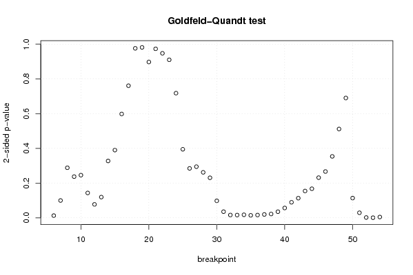
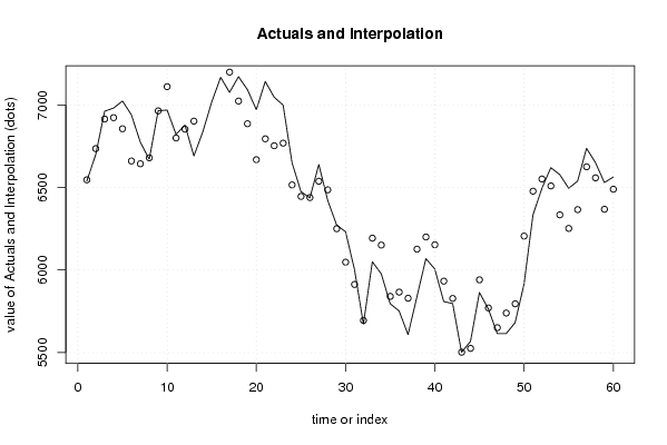
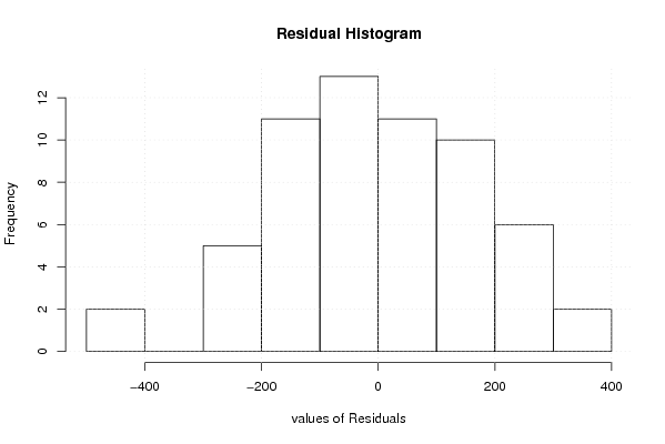
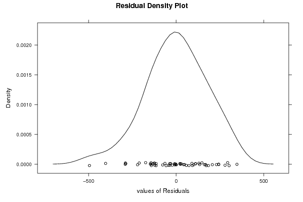
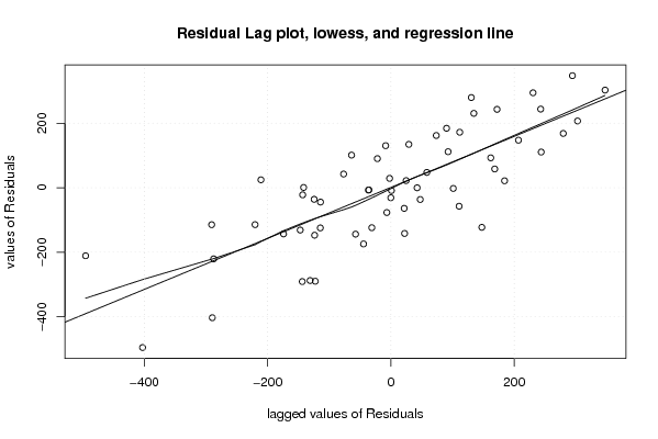
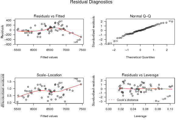
library(lattice) library(lmtest) n25 <- 25 #minimum number of obs. for Goldfeld-Quandt test par1 <- as.numeric(par1) x <- t(y) k <- length(x[1,]) n <- length(x[,1]) x1 <- cbind(x[,par1], x[,1:k!=par1]) mycolnames <- c(colnames(x)[par1], colnames(x)[1:k!=par1]) colnames(x1) <- mycolnames #colnames(x)[par1] x <- x1 if (par3 == 'First Differences'){ x2 <- array(0, dim=c(n-1,k), dimnames=list(1:(n-1), paste('(1-B)',colnames(x),sep=''))) for (i in 1:n-1) { for (j in 1:k) { x2[i,j] <- x[i+1,j] - x[i,j] } } x <- x2 } if (par2 == 'Include Monthly Dummies'){ x2 <- array(0, dim=c(n,11), dimnames=list(1:n, paste('M', seq(1:11), sep =''))) for (i in 1:11){ x2[seq(i,n,12),i] <- 1 } x <- cbind(x, x2) } if (par2 == 'Include Quarterly Dummies'){ x2 <- array(0, dim=c(n,3), dimnames=list(1:n, paste('Q', seq(1:3), sep =''))) for (i in 1:3){ x2[seq(i,n,4),i] <- 1 } x <- cbind(x, x2) } k <- length(x[1,]) if (par3 == 'Linear Trend'){ x <- cbind(x, c(1:n)) colnames(x)[k+1] <- 't' } x k <- length(x[1,]) df <- as.data.frame(x) (mylm <- lm(df)) (mysum <- summary(mylm)) if (n > n25) { kp3 <- k + 3 nmkm3 <- n - k - 3 gqarr <- array(NA, dim=c(nmkm3-kp3+1,3)) numgqtests <- 0 numsignificant1 <- 0 numsignificant5 <- 0 numsignificant10 <- 0 for (mypoint in kp3:nmkm3) { j <- 0 numgqtests <- numgqtests + 1 for (myalt in c('greater', 'two.sided', 'less')) { j <- j + 1 gqarr[mypoint-kp3+1,j] <- gqtest(mylm, point=mypoint, alternative=myalt)$p.value } if (gqarr[mypoint-kp3+1,2] < 0.01) numsignificant1 <- numsignificant1 + 1 if (gqarr[mypoint-kp3+1,2] < 0.05) numsignificant5 <- numsignificant5 + 1 if (gqarr[mypoint-kp3+1,2] < 0.10) numsignificant10 <- numsignificant10 + 1 } gqarr } bitmap(file='test0.png') plot(x[,1], type='l', main='Actuals and Interpolation', ylab='value of Actuals and Interpolation (dots)', xlab='time or index') points(x[,1]-mysum$resid) grid() dev.off() bitmap(file='test1.png') plot(mysum$resid, type='b', pch=19, main='Residuals', ylab='value of Residuals', xlab='time or index') grid() dev.off() bitmap(file='test2.png') hist(mysum$resid, main='Residual Histogram', xlab='values of Residuals') grid() dev.off() bitmap(file='test3.png') densityplot(~mysum$resid,col='black',main='Residual Density Plot', xlab='values of Residuals') dev.off() bitmap(file='test4.png') qqnorm(mysum$resid, main='Residual Normal Q-Q Plot') qqline(mysum$resid) grid() dev.off() (myerror <- as.ts(mysum$resid)) bitmap(file='test5.png') dum <- cbind(lag(myerror,k=1),myerror) dum dum1 <- dum[2:length(myerror),] dum1 z <- as.data.frame(dum1) z plot(z,main=paste('Residual Lag plot, lowess, and regression line'), ylab='values of Residuals', xlab='lagged values of Residuals') lines(lowess(z)) abline(lm(z)) grid() dev.off() bitmap(file='test6.png') acf(mysum$resid, lag.max=length(mysum$resid)/2, main='Residual Autocorrelation Function') grid() dev.off() bitmap(file='test7.png') pacf(mysum$resid, lag.max=length(mysum$resid)/2, main='Residual Partial Autocorrelation Function') grid() dev.off() bitmap(file='test8.png') opar <- par(mfrow = c(2,2), oma = c(0, 0, 1.1, 0)) plot(mylm, las = 1, sub='Residual Diagnostics') par(opar) dev.off() if (n > n25) { bitmap(file='test9.png') plot(kp3:nmkm3,gqarr[,2], main='Goldfeld-Quandt test',ylab='2-sided p-value',xlab='breakpoint') grid() dev.off() } load(file='createtable') a<-table.start() a<-table.row.start(a) a<-table.element(a, 'Multiple Linear Regression - Estimated Regression Equation', 1, TRUE) a<-table.row.end(a) myeq <- colnames(x)[1] myeq <- paste(myeq, '[t] = ', sep='') for (i in 1:k){ if (mysum$coefficients[i,1] > 0) myeq <- paste(myeq, '+', '') myeq <- paste(myeq, mysum$coefficients[i,1], sep=' ') if (rownames(mysum$coefficients)[i] != '(Intercept)') { myeq <- paste(myeq, rownames(mysum$coefficients)[i], sep='') if (rownames(mysum$coefficients)[i] != 't') myeq <- paste(myeq, '[t]', sep='') } } myeq <- paste(myeq, ' + e[t]') a<-table.row.start(a) a<-table.element(a, myeq) a<-table.row.end(a) a<-table.end(a) table.save(a,file='mytable1.tab') a<-table.start() a<-table.row.start(a) a<-table.element(a,hyperlink('http://www.xycoon.com/ols1.htm','Multiple Linear Regression - Ordinary Least Squares',''), 6, TRUE) a<-table.row.end(a) a<-table.row.start(a) a<-table.element(a,'Variable',header=TRUE) a<-table.element(a,'Parameter',header=TRUE) a<-table.element(a,'S.D.',header=TRUE) a<-table.element(a,'T-STAT<br />H0: parameter = 0',header=TRUE) a<-table.element(a,'2-tail p-value',header=TRUE) a<-table.element(a,'1-tail p-value',header=TRUE) a<-table.row.end(a) for (i in 1:k){ a<-table.row.start(a) a<-table.element(a,rownames(mysum$coefficients)[i],header=TRUE) a<-table.element(a,mysum$coefficients[i,1]) a<-table.element(a, round(mysum$coefficients[i,2],6)) a<-table.element(a, round(mysum$coefficients[i,3],4)) a<-table.element(a, round(mysum$coefficients[i,4],6)) a<-table.element(a, round(mysum$coefficients[i,4]/2,6)) a<-table.row.end(a) } a<-table.end(a) table.save(a,file='mytable2.tab') a<-table.start() a<-table.row.start(a) a<-table.element(a, 'Multiple Linear Regression - Regression Statistics', 2, TRUE) a<-table.row.end(a) a<-table.row.start(a) a<-table.element(a, 'Multiple R',1,TRUE) a<-table.element(a, sqrt(mysum$r.squared)) a<-table.row.end(a) a<-table.row.start(a) a<-table.element(a, 'R-squared',1,TRUE) a<-table.element(a, mysum$r.squared) a<-table.row.end(a) a<-table.row.start(a) a<-table.element(a, 'Adjusted R-squared',1,TRUE) a<-table.element(a, mysum$adj.r.squared) a<-table.row.end(a) a<-table.row.start(a) a<-table.element(a, 'F-TEST (value)',1,TRUE) a<-table.element(a, mysum$fstatistic[1]) a<-table.row.end(a) a<-table.row.start(a) a<-table.element(a, 'F-TEST (DF numerator)',1,TRUE) a<-table.element(a, mysum$fstatistic[2]) a<-table.row.end(a) a<-table.row.start(a) a<-table.element(a, 'F-TEST (DF denominator)',1,TRUE) a<-table.element(a, mysum$fstatistic[3]) a<-table.row.end(a) a<-table.row.start(a) a<-table.element(a, 'p-value',1,TRUE) a<-table.element(a, 1-pf(mysum$fstatistic[1],mysum$fstatistic[2],mysum$fstatistic[3])) a<-table.row.end(a) a<-table.row.start(a) a<-table.element(a, 'Multiple Linear Regression - Residual Statistics', 2, TRUE) a<-table.row.end(a) a<-table.row.start(a) a<-table.element(a, 'Residual Standard Deviation',1,TRUE) a<-table.element(a, mysum$sigma) a<-table.row.end(a) a<-table.row.start(a) a<-table.element(a, 'Sum Squared Residuals',1,TRUE) a<-table.element(a, sum(myerror*myerror)) a<-table.row.end(a) a<-table.end(a) table.save(a,file='mytable3.tab') a<-table.start() a<-table.row.start(a) a<-table.element(a, 'Multiple Linear Regression - Actuals, Interpolation, and Residuals', 4, TRUE) a<-table.row.end(a) a<-table.row.start(a) a<-table.element(a, 'Time or Index', 1, TRUE) a<-table.element(a, 'Actuals', 1, TRUE) a<-table.element(a, 'Interpolation<br />Forecast', 1, TRUE) a<-table.element(a, 'Residuals<br />Prediction Error', 1, TRUE) a<-table.row.end(a) for (i in 1:n) { a<-table.row.start(a) a<-table.element(a,i, 1, TRUE) a<-table.element(a,x[i]) a<-table.element(a,x[i]-mysum$resid[i]) a<-table.element(a,mysum$resid[i]) a<-table.row.end(a) } a<-table.end(a) table.save(a,file='mytable4.tab') if (n > n25) { a<-table.start() a<-table.row.start(a) a<-table.element(a,'Goldfeld-Quandt test for Heteroskedasticity',4,TRUE) a<-table.row.end(a) a<-table.row.start(a) a<-table.element(a,'p-values',header=TRUE) a<-table.element(a,'Alternative Hypothesis',3,header=TRUE) a<-table.row.end(a) a<-table.row.start(a) a<-table.element(a,'breakpoint index',header=TRUE) a<-table.element(a,'greater',header=TRUE) a<-table.element(a,'2-sided',header=TRUE) a<-table.element(a,'less',header=TRUE) a<-table.row.end(a) for (mypoint in kp3:nmkm3) { a<-table.row.start(a) a<-table.element(a,mypoint,header=TRUE) a<-table.element(a,gqarr[mypoint-kp3+1,1]) a<-table.element(a,gqarr[mypoint-kp3+1,2]) a<-table.element(a,gqarr[mypoint-kp3+1,3]) a<-table.row.end(a) } a<-table.end(a) table.save(a,file='mytable5.tab') a<-table.start() a<-table.row.start(a) a<-table.element(a,'Meta Analysis of Goldfeld-Quandt test for Heteroskedasticity',4,TRUE) a<-table.row.end(a) a<-table.row.start(a) a<-table.element(a,'Description',header=TRUE) a<-table.element(a,'# significant tests',header=TRUE) a<-table.element(a,'% significant tests',header=TRUE) a<-table.element(a,'OK/NOK',header=TRUE) a<-table.row.end(a) a<-table.row.start(a) a<-table.element(a,'1% type I error level',header=TRUE) a<-table.element(a,numsignificant1) a<-table.element(a,numsignificant1/numgqtests) if (numsignificant1/numgqtests < 0.01) dum <- 'OK' else dum <- 'NOK' a<-table.element(a,dum) a<-table.row.end(a) a<-table.row.start(a) a<-table.element(a,'5% type I error level',header=TRUE) a<-table.element(a,numsignificant5) a<-table.element(a,numsignificant5/numgqtests) if (numsignificant5/numgqtests < 0.05) dum <- 'OK' else dum <- 'NOK' a<-table.element(a,dum) a<-table.row.end(a) a<-table.row.start(a) a<-table.element(a,'10% type I error level',header=TRUE) a<-table.element(a,numsignificant10) a<-table.element(a,numsignificant10/numgqtests) if (numsignificant10/numgqtests < 0.1) dum <- 'OK' else dum <- 'NOK' a<-table.element(a,dum) a<-table.row.end(a) a<-table.end(a) table.save(a,file='mytable6.tab') }

Copyright

This work is licensed under a Creative Commons Attribution-Noncommercial-Share Alike 3.0 License.

Software written by Ed van Stee & Patrick Wessa

Disclaimer

Information provided on this web site is provided "AS IS" without warranty of any kind, either express or implied, including, without limitation, warranties of merchantability, fitness for a particular purpose, and noninfringement. We use reasonable efforts to include accurate and timely information and periodically update the information, and software without notice. However, we make no warranties or representations as to the accuracy or completeness of such information (or software), and we assume no liability or responsibility for errors or omissions in the content of this web site, or any software bugs in online applications. Your use of this web site is AT YOUR OWN RISK. Under no circumstances and under no legal theory shall we be liable to you or any other person for any direct, indirect, special, incidental, exemplary, or consequential damages arising from your access to, or use of, this web site.

Privacy Policy

We may request personal information to be submitted to our servers in order to be able to:

• personalize online software applications according to your needs
• enforce strict security rules with respect to the data that you upload (e.g. statistical data)
• manage user sessions of online applications
• alert you about important changes or upgrades in resources or applications

We NEVER allow other companies to directly offer registered users information about their products and services. Banner references and hyperlinks of third parties NEVER contain any personal data of the visitor.

We do NOT sell, nor transmit by any means, personal information, nor statistical data series uploaded by you to third parties.

We carefully protect your data from loss, misuse, alteration, and destruction. However, at any time, and under any circumstance you are solely responsible for managing your passwords, and keeping them secret.

We store a unique ANONYMOUS USER ID in the form of a small 'Cookie' on your computer. This allows us to track your progress when using this website which is necessary to create state-dependent features. The cookie is used for NO OTHER PURPOSE. At any time you may opt to disallow cookies from this website - this will not affect other features of this website.

We examine cookies that are used by third-parties (banner and online ads) very closely: abuse from third-parties automatically results in termination of the advertising contract without refund. We have very good reason to believe that the cookies that are produced by third parties (banner ads) do NOT cause any privacy or security risk.

FreeStatistics.org is safe. There is no need to download any software to use the applications and services contained in this website. Hence, your system's security is not compromised by their use, and your personal data - other than data you submit in the account application form, and the user-agent information that is transmitted by your browser - is never transmitted to our servers.

As a general rule, we do not log on-line behavior of individuals (other than normal logging of webserver 'hits'). However, in cases of abuse, hacking, unauthorized access, Denial of Service attacks, illegal copying, hotlinking, non-compliance with international webstandards (such as robots.txt), or any other harmful behavior, our system engineers are empowered to log, track, identify, publish, and ban misbehaving individuals - even if this leads to ban entire blocks of IP addresses, or disclosing user's identity.

FreeStatistics.org is powered by