*The author of this computation has been verified*

R Software Module: /rwasp_centraltendency.wasp (opens new window with default values)

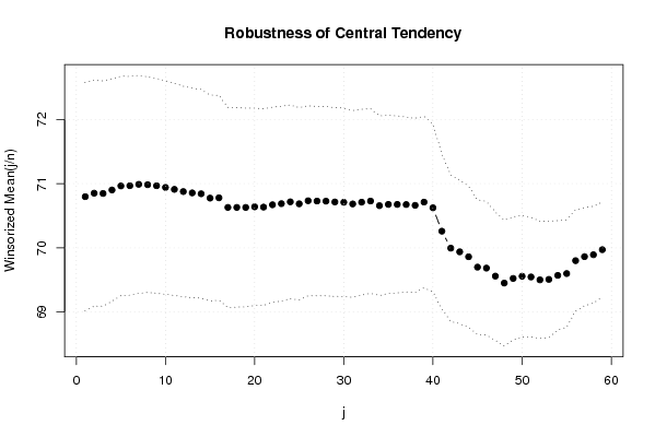
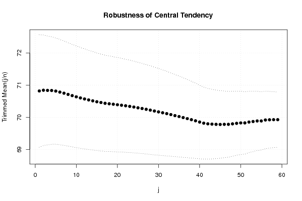
Title produced by software: Central Tendency

Date of computation: Wed, 24 Nov 2010 19:07:18 +0000

Cite this page as follows:

Statistical Computations at FreeStatistics.org, Office for Research Development and Education, URL http://www.freestatistics.org/blog/date/2010/Nov/24/t1290625551oqj2rpv2uw3isz7.htm/, Retrieved Wed, 24 Nov 2010 20:05:53 +0100

BibTeX entries for LaTeX users:

@Manual{KEY, author = {{YOUR NAME}}, publisher = {Office for Research Development and Education}, title = {Statistical Computations at FreeStatistics.org, URL http://www.freestatistics.org/blog/date/2010/Nov/24/t1290625551oqj2rpv2uw3isz7.htm/}, year = {2010}, } @Manual{R, title = {R: A Language and Environment for Statistical Computing}, author = {{R Development Core Team}}, organization = {R Foundation for Statistical Computing}, address = {Vienna, Austria}, year = {2010}, note = {{ISBN} 3-900051-07-0}, url = {http://www.R-project.org}, }

Original text written by user:

IsPrivate?

No (this computation is public)

User-defined keywords:

Dataseries X:

» Textbox « » Textfile « » CSV «

64.033 65.679 62.776 67.024 67.988 69.529 70.158 69.410 74.049 66.197 67.043 67.459 65.512 64.665 65.382 66.607 58.387 57.564 58.431 65.012 64.176 65.509 65.163 62.158 64.429 61.325 65.339 69.921 70.782 73.287 70.300 71.579 70.700 75.740 75.850 76.381 77.388 75.519 75.573 76.668 79.387 76.876 81.021 82.883 84.016 85.047 85.757 84.792 83.811 84.691 83.496 85.470 85.212 84.802 85.809 85.119 85.228 85.302 85.883 86.315 86.195 88.227 86.411 89.120 88.030 89.372 91.869 92.845 92.787 94.711 94.204 97.217 95.118 93.688 93.140 91.516 90.957 90.372 89.749 85.813 86.026 83.933 83.602 83.384 76.369 60.808 48.071 42.604 41.402 62.121 79.739 79.006 74.472 75.956 75.041 74.873 72.922 70.472 71.423 71.363 73.297 72.081 70.488 65.544 64.450 61.698 61.352 61.072 63.722 61.987 53.802 47.818 50.998 58.438 60.143 61.854 70.987 70.389 72.175 70.243 69.616 69.443 70.833 71.059 72.218 72.647 73.299 73.756 etc...

Output produced by software:

Summary of computational transaction Raw Input view raw input (R code) Raw Output view raw output of R engine Computing time 2 seconds R Server 'Gwilym Jenkins' @ 72.249.127.135 Central Tendency - Ungrouped Data Measure Value S.E. Value/S.E. Arithmetic Mean 70.8024831460674 0.892643010020997 79.3178038154379 Geometric Mean 69.8015026621748 Harmonic Mean 68.7950752316655 Quadratic Mean 71.7915542582846 Winsorized Mean ( 1 / 59 ) 70.7974438202247 0.889513443975888 79.5912015717031 Winsorized Mean ( 2 / 59 ) 70.8514550561798 0.8792235528029 80.5841186013621 Winsorized Mean ( 3 / 59 ) 70.8471741573034 0.877297572136642 80.7561498030325 Winsorized Mean ( 4 / 59 ) 70.9013539325843 0.866468634981841 81.827952068998 Winsorized Mean ( 5 / 59 ) 70.9647247191011 0.854613047956678 83.0372586620026 Winsorized Mean ( 6 / 59 ) 70.9675561797753 0.851726623898028 83.3219887561855 Winsorized Mean ( 7 / 59 ) 70.990011235955 0.848686230688885 83.6469459134879 Winsorized Mean ( 8 / 59 ) 70.9837191011236 0.839095567702088 84.595511921862 Winsorized Mean ( 9 / 59 ) 70.9670337078652 0.836481430352007 84.839939217779 Winsorized Mean ( 10 / 59 ) 70.941415730337 0.83156726510729 85.310495863716 Winsorized Mean ( 11 / 59 ) 70.9114438202247 0.82606445205833 85.8425073776417 Winsorized Mean ( 12 / 59 ) 70.8771966292135 0.819738147396098 86.4632161554945 Winsorized Mean ( 13 / 59 ) 70.856308988764 0.815497613786025 86.8872057881407 Winsorized Mean ( 14 / 59 ) 70.8422303370786 0.812377111744627 87.2036266321449 Winsorized Mean ( 15 / 59 ) 70.7750674157303 0.802137798534779 88.2330536536382 Winsorized Mean ( 16 / 59 ) 70.7796516853933 0.79769033557258 88.7307373914563 Winsorized Mean ( 17 / 59 ) 70.6299943820225 0.778880706518125 90.6814019026916 Winsorized Mean ( 18 / 59 ) 70.6301966292135 0.776756940881659 90.9295983233116 Winsorized Mean ( 19 / 59 ) 70.6296629213483 0.774047821286265 91.2471568022506 Winsorized Mean ( 20 / 59 ) 70.6391011235955 0.769022021295205 91.8557585706368 Winsorized Mean ( 21 / 59 ) 70.6348539325843 0.765853070301668 92.2302941277774 Winsorized Mean ( 22 / 59 ) 70.6713146067416 0.760401561940933 92.939465335069 Winsorized Mean ( 23 / 59 ) 70.6885 0.758607244362833 93.181946949864 Winsorized Mean ( 24 / 59 ) 70.7168146067416 0.754385894480379 93.740902532982 Winsorized Mean ( 25 / 59 ) 70.6860561797753 0.748946127497109 94.380695198999 Winsorized Mean ( 26 / 59 ) 70.7335280898876 0.739339850670549 95.6711964406293 Winsorized Mean ( 27 / 59 ) 70.7289775280899 0.737462394525987 95.9085887675016 Winsorized Mean ( 28 / 59 ) 70.7275617977528 0.737079163064775 95.9565340358661 Winsorized Mean ( 29 / 59 ) 70.714691011236 0.735184565703488 96.186310635575 Winsorized Mean ( 30 / 59 ) 70.7098033707865 0.733160046716525 96.4452491477981 Winsorized Mean ( 31 / 59 ) 70.6840280898876 0.726872896328066 97.2440002192422 Winsorized Mean ( 32 / 59 ) 70.7115337078652 0.723931228465677 97.6771424237817 Winsorized Mean ( 33 / 59 ) 70.7291460674157 0.718496521397389 98.4404850420933 Winsorized Mean ( 34 / 59 ) 70.6571348314607 0.699199171385321 101.054374380147 Winsorized Mean ( 35 / 59 ) 70.676797752809 0.694132717087736 101.820294610714 Winsorized Mean ( 36 / 59 ) 70.676797752809 0.689219315824526 102.546165103131 Winsorized Mean ( 37 / 59 ) 70.6747191011236 0.680789805600436 103.812834034421 Winsorized Mean ( 38 / 59 ) 70.6623370786517 0.677436458048693 104.308435483661 Winsorized Mean ( 39 / 59 ) 70.7127303370787 0.668065375637992 105.84702173728 Winsorized Mean ( 40 / 59 ) 70.624191011236 0.65391812647094 108.001580247331 Winsorized Mean ( 41 / 59 ) 70.2602584269663 0.603699618956336 116.382810624315 Winsorized Mean ( 42 / 59 ) 69.9950449438202 0.570439851618129 122.703637807334 Winsorized Mean ( 43 / 59 ) 69.9385168539326 0.55965367740727 124.967492714315 Winsorized Mean ( 44 / 59 ) 69.861393258427 0.549157043017766 127.215692025945 Winsorized Mean ( 45 / 59 ) 69.6998483146067 0.525055247367535 132.747646393518 Winsorized Mean ( 46 / 59 ) 69.6846011235955 0.520344303521054 133.92017679843 Winsorized Mean ( 47 / 59 ) 69.5599719101124 0.500361851126212 139.019335214200 Winsorized Mean ( 48 / 59 ) 69.4515674157303 0.489557922896617 141.865883825961 Winsorized Mean ( 49 / 59 ) 69.5239662921348 0.478726392879522 145.226934061334 Winsorized Mean ( 50 / 59 ) 69.5579550561798 0.47383676741792 146.797293581125 Winsorized Mean ( 51 / 59 ) 69.5464943820225 0.466048603660862 149.225840042706 Winsorized Mean ( 52 / 59 ) 69.501797752809 0.455263749763264 152.662709888388 Winsorized Mean ( 53 / 59 ) 69.5092415730337 0.453950201307027 153.120851963278 Winsorized Mean ( 54 / 59 ) 69.5714325842697 0.426275793033536 163.207561210956 Winsorized Mean ( 55 / 59 ) 69.5998595505618 0.418011990917154 166.502064684446 Winsorized Mean ( 56 / 59 ) 69.8005786516854 0.394284008915367 177.031218800122 Winsorized Mean ( 57 / 59 ) 69.8630224719101 0.382496989768299 182.649862196903 Winsorized Mean ( 58 / 59 ) 69.893 0.377080918598318 185.352789156783 Winsorized Mean ( 59 / 59 ) 69.9715561797753 0.369483279797564 189.376786462738 Trimmed Mean ( 1 / 59 ) 70.8194488636364 0.874274814805527 81.0036474393802 Trimmed Mean ( 2 / 59 ) 70.841959770115 0.857913860267475 82.5746768422978 Trimmed Mean ( 3 / 59 ) 70.8370465116279 0.846102122661876 83.7216272295492 Trimmed Mean ( 4 / 59 ) 70.8335117647059 0.834168759505156 84.9150857755997 Trimmed Mean ( 5 / 59 ) 70.8155416666667 0.824567148454676 85.882079827437 Trimmed Mean ( 6 / 59 ) 70.7835481927711 0.817112757849443 86.6264141794409 Trimmed Mean ( 7 / 59 ) 70.750262195122 0.809680612842138 87.380457272868 Trimmed Mean ( 8 / 59 ) 70.7126296296296 0.802216310199272 88.1465868128067 Trimmed Mean ( 9 / 59 ) 70.67493125 0.795736565560857 88.8169958611697 Trimmed Mean ( 10 / 59 ) 70.6383670886076 0.789122212761587 89.515116855479 Trimmed Mean ( 11 / 59 ) 70.6037884615385 0.782650743744619 90.2111050501687 Trimmed Mean ( 12 / 59 ) 70.571461038961 0.776358649124036 90.9005922953092 Trimmed Mean ( 13 / 59 ) 70.541625 0.770312088189759 91.5753836419386 Trimmed Mean ( 14 / 59 ) 70.5129 0.764236682405249 92.2657883655595 Trimmed Mean ( 15 / 59 ) 70.4846081081081 0.757975720113265 92.990588270526 Trimmed Mean ( 16 / 59 ) 70.461 0.752265523066253 93.6650661761013 Trimmed Mean ( 17 / 59 ) 70.4363819444444 0.746487037362294 94.3571400694791 Trimmed Mean ( 18 / 59 ) 70.4221056338028 0.742054065894388 94.9015831466727 Trimmed Mean ( 19 / 59 ) 70.4074071428571 0.737380102323638 95.4831937029339 Trimmed Mean ( 20 / 59 ) 70.3923188405797 0.732490044787678 96.1000348625678 Trimmed Mean ( 21 / 59 ) 70.376169117647 0.72756374654681 96.728526471624 Trimmed Mean ( 22 / 59 ) 70.3598059701493 0.722417968015372 97.394872615699 Trimmed Mean ( 23 / 59 ) 70.3407121212121 0.717215688239685 98.0746981341896 Trimmed Mean ( 24 / 59 ) 70.3200076923077 0.711621232030568 98.8166239667328 Trimmed Mean ( 25 / 59 ) 70.297015625 0.70579799224309 99.5993420179473 Trimmed Mean ( 26 / 59 ) 70.2750317460317 0.699833284177547 100.416818312121 Trimmed Mean ( 27 / 59 ) 70.2497177419355 0.694032949454089 101.219571487481 Trimmed Mean ( 28 / 59 ) 70.2238196721311 0.687753449533624 102.106095897812 Trimmed Mean ( 29 / 59 ) 70.1971333333333 0.680812478648196 103.107882911775 Trimmed Mean ( 30 / 59 ) 70.1702118644068 0.673270455652081 104.222918554246 Trimmed Mean ( 31 / 59 ) 70.1426120689655 0.665065680129632 105.467195443454 Trimmed Mean ( 32 / 59 ) 70.1153421052632 0.656500333045671 106.801685507120 Trimmed Mean ( 33 / 59 ) 70.0857321428571 0.647207640722421 108.289407808330 Trimmed Mean ( 34 / 59 ) 70.0541818181818 0.637321486322047 109.919692528274 Trimmed Mean ( 35 / 59 ) 70.0249537037037 0.628055408204054 111.494866199692 Trimmed Mean ( 36 / 59 ) 69.993679245283 0.61812672798573 113.235160487833 Trimmed Mean ( 37 / 59 ) 69.961201923077 0.607439463568705 115.173949206486 Trimmed Mean ( 38 / 59 ) 69.9275490196078 0.596220903588623 117.284631583223 Trimmed Mean ( 39 / 59 ) 69.89313 0.583907086087186 119.69906114406 Trimmed Mean ( 40 / 59 ) 69.8549591836735 0.570891565403121 122.361168770022 Trimmed Mean ( 41 / 59 ) 69.8193020833333 0.557648332308338 125.203103888650 Trimmed Mean ( 42 / 59 ) 69.7989361702128 0.547899063142542 127.393786311428 Trimmed Mean ( 43 / 59 ) 69.789902173913 0.540136047314161 129.208006984435 Trimmed Mean ( 44 / 59 ) 69.7830666666667 0.532316728157358 131.093131166898 Trimmed Mean ( 45 / 59 ) 69.7794659090909 0.524397043901149 133.06609318386 Trimmed Mean ( 46 / 59 ) 69.7831279069767 0.517687824264448 134.797699764578 Trimmed Mean ( 47 / 59 ) 69.7831279069767 0.510389573496169 136.725222321769 Trimmed Mean ( 48 / 59 ) 69.7981829268293 0.503943769813667 138.503910768928 Trimmed Mean ( 49 / 59 ) 69.81425 0.497487654099087 140.333633256545 Trimmed Mean ( 50 / 59 ) 69.8277692307692 0.491080241749949 142.192178170191 Trimmed Mean ( 51 / 59 ) 69.8277692307692 0.48406669838296 144.25237155134 Trimmed Mean ( 52 / 59 ) 69.8542702702703 0.47665240762651 146.551804108385 Trimmed Mean ( 53 / 59 ) 69.8710277777778 0.469095603309075 148.948374883278 Trimmed Mean ( 54 / 59 ) 69.8883857142857 0.460255480990418 151.846938495754 Trimmed Mean ( 55 / 59 ) 69.8883857142857 0.453196999986486 154.211933698523 Trimmed Mean ( 56 / 59 ) 69.9186515151515 0.445739103603573 156.860035276006 Trimmed Mean ( 57 / 59 ) 69.924515625 0.439849918032219 158.973578846678 Trimmed Mean ( 58 / 59 ) 69.9276129032258 0.434154022385228 161.066371144153 Trimmed Mean ( 59 / 59 ) 69.9276129032258 0.427816842701695 163.452220491432 Median 70.3445 Midrange 69.3095 Midmean - Weighted Average at Xnp 69.6794382022472 Midmean - Weighted Average at X(n+1)p 69.7830666666667 Midmean - Empirical Distribution Function 69.7830666666667 Midmean - Empirical Distribution Function - Averaging 69.7830666666667 Midmean - Empirical Distribution Function - Interpolation 69.7794659090909 Midmean - Closest Observation 69.7830666666667 Midmean - True Basic - Statistics Graphics Toolkit 69.7830666666667 Midmean - MS Excel (old versions) 69.7830666666667 Number of observations 178

Charts produced by software:

http://www.freestatistics.org/blog/date/2010/Nov/24/t1290625551oqj2rpv2uw3isz7/1fdq91290625635.png (open in new window) http://www.freestatistics.org/blog/date/2010/Nov/24/t1290625551oqj2rpv2uw3isz7/1fdq91290625635.ps (open in new window) http://www.freestatistics.org/blog/date/2010/Nov/24/t1290625551oqj2rpv2uw3isz7/2qn7c1290625635.png (open in new window) http://www.freestatistics.org/blog/date/2010/Nov/24/t1290625551oqj2rpv2uw3isz7/2qn7c1290625635.ps (open in new window)

Parameters (Session):

Parameters (R input):

R code (references can be found in the software module):

geomean <- function(x) { return(exp(mean(log(x)))) } harmean <- function(x) { return(1/mean(1/x)) } quamean <- function(x) { return(sqrt(mean(x*x))) } winmean <- function(x) { x <-sort(x[!is.na(x)]) n<-length(x) denom <- 3 nodenom <- n/denom if (nodenom>40) denom <- n/40 sqrtn = sqrt(n) roundnodenom = floor(nodenom) win <- array(NA,dim=c(roundnodenom,2)) for (j in 1:roundnodenom) { win[j,1] <- (j*x[j+1]+sum(x[(j+1):(n-j)])+j*x[n-j])/n win[j,2] <- sd(c(rep(x[j+1],j),x[(j+1):(n-j)],rep(x[n-j],j)))/sqrtn } return(win) } trimean <- function(x) { x <-sort(x[!is.na(x)]) n<-length(x) denom <- 3 nodenom <- n/denom if (nodenom>40) denom <- n/40 sqrtn = sqrt(n) roundnodenom = floor(nodenom) tri <- array(NA,dim=c(roundnodenom,2)) for (j in 1:roundnodenom) { tri[j,1] <- mean(x,trim=j/n) tri[j,2] <- sd(x[(j+1):(n-j)]) / sqrt(n-j*2) } return(tri) } midrange <- function(x) { return((max(x)+min(x))/2) } q1 <- function(data,n,p,i,f) { np <- n*p; i <<- floor(np) f <<- np - i qvalue <- (1-f)*data[i] + f*data[i+1] } q2 <- function(data,n,p,i,f) { np <- (n+1)*p i <<- floor(np) f <<- np - i qvalue <- (1-f)*data[i] + f*data[i+1] } q3 <- function(data,n,p,i,f) { np <- n*p i <<- floor(np) f <<- np - i if (f==0) { qvalue <- data[i] } else { qvalue <- data[i+1] } } q4 <- function(data,n,p,i,f) { np <- n*p i <<- floor(np) f <<- np - i if (f==0) { qvalue <- (data[i]+data[i+1])/2 } else { qvalue <- data[i+1] } } q5 <- function(data,n,p,i,f) { np <- (n-1)*p i <<- floor(np) f <<- np - i if (f==0) { qvalue <- data[i+1] } else { qvalue <- data[i+1] + f*(data[i+2]-data[i+1]) } } q6 <- function(data,n,p,i,f) { np <- n*p+0.5 i <<- floor(np) f <<- np - i qvalue <- data[i] } q7 <- function(data,n,p,i,f) { np <- (n+1)*p i <<- floor(np) f <<- np - i if (f==0) { qvalue <- data[i] } else { qvalue <- f*data[i] + (1-f)*data[i+1] } } q8 <- function(data,n,p,i,f) { np <- (n+1)*p i <<- floor(np) f <<- np - i if (f==0) { qvalue <- data[i] } else { if (f == 0.5) { qvalue <- (data[i]+data[i+1])/2 } else { if (f < 0.5) { qvalue <- data[i] } else { qvalue <- data[i+1] } } } } midmean <- function(x,def) { x <-sort(x[!is.na(x)]) n<-length(x) if (def==1) { qvalue1 <- q1(x,n,0.25,i,f) qvalue3 <- q1(x,n,0.75,i,f) } if (def==2) { qvalue1 <- q2(x,n,0.25,i,f) qvalue3 <- q2(x,n,0.75,i,f) } if (def==3) { qvalue1 <- q3(x,n,0.25,i,f) qvalue3 <- q3(x,n,0.75,i,f) } if (def==4) { qvalue1 <- q4(x,n,0.25,i,f) qvalue3 <- q4(x,n,0.75,i,f) } if (def==5) { qvalue1 <- q5(x,n,0.25,i,f) qvalue3 <- q5(x,n,0.75,i,f) } if (def==6) { qvalue1 <- q6(x,n,0.25,i,f) qvalue3 <- q6(x,n,0.75,i,f) } if (def==7) { qvalue1 <- q7(x,n,0.25,i,f) qvalue3 <- q7(x,n,0.75,i,f) } if (def==8) { qvalue1 <- q8(x,n,0.25,i,f) qvalue3 <- q8(x,n,0.75,i,f) } midm <- 0 myn <- 0 roundno4 <- round(n/4) round3no4 <- round(3*n/4) for (i in 1:n) { if ((x[i]>=qvalue1) & (x[i]<=qvalue3)){ midm = midm + x[i] myn = myn + 1 } } midm = midm / myn return(midm) } (arm <- mean(x)) sqrtn <- sqrt(length(x)) (armse <- sd(x) / sqrtn) (armose <- arm / armse) (geo <- geomean(x)) (har <- harmean(x)) (qua <- quamean(x)) (win <- winmean(x)) (tri <- trimean(x)) (midr <- midrange(x)) midm <- array(NA,dim=8) for (j in 1:8) midm[j] <- midmean(x,j) midm bitmap(file='test1.png') lb <- win[,1] - 2*win[,2] ub <- win[,1] + 2*win[,2] if ((ylimmin == '') | (ylimmax == '')) plot(win[,1],type='b',main=main, xlab='j', pch=19, ylab='Winsorized Mean(j/n)', ylim=c(min(lb),max(ub))) else plot(win[,1],type='l',main=main, xlab='j', pch=19, ylab='Winsorized Mean(j/n)', ylim=c(ylimmin,ylimmax)) lines(ub,lty=3) lines(lb,lty=3) grid() dev.off() bitmap(file='test2.png') lb <- tri[,1] - 2*tri[,2] ub <- tri[,1] + 2*tri[,2] if ((ylimmin == '') | (ylimmax == '')) plot(tri[,1],type='b',main=main, xlab='j', pch=19, ylab='Trimmed Mean(j/n)', ylim=c(min(lb),max(ub))) else plot(tri[,1],type='l',main=main, xlab='j', pch=19, ylab='Trimmed Mean(j/n)', ylim=c(ylimmin,ylimmax)) lines(ub,lty=3) lines(lb,lty=3) grid() dev.off() load(file='createtable') a<-table.start() a<-table.row.start(a) a<-table.element(a,'Central Tendency - Ungrouped Data',4,TRUE) a<-table.row.end(a) a<-table.row.start(a) a<-table.element(a,'Measure',header=TRUE) a<-table.element(a,'Value',header=TRUE) a<-table.element(a,'S.E.',header=TRUE) a<-table.element(a,'Value/S.E.',header=TRUE) a<-table.row.end(a) a<-table.row.start(a) a<-table.element(a,hyperlink('http://www.xycoon.com/arithmetic_mean.htm', 'Arithmetic Mean', 'click to view the definition of the Arithmetic Mean'),header=TRUE) a<-table.element(a,arm) a<-table.element(a,hyperlink('http://www.xycoon.com/arithmetic_mean_standard_error.htm', armse, 'click to view the definition of the Standard Error of the Arithmetic Mean')) a<-table.element(a,armose) a<-table.row.end(a) a<-table.row.start(a) a<-table.element(a,hyperlink('http://www.xycoon.com/geometric_mean.htm', 'Geometric Mean', 'click to view the definition of the Geometric Mean'),header=TRUE) a<-table.element(a,geo) a<-table.element(a,'') a<-table.element(a,'') a<-table.row.end(a) a<-table.row.start(a) a<-table.element(a,hyperlink('http://www.xycoon.com/harmonic_mean.htm', 'Harmonic Mean', 'click to view the definition of the Harmonic Mean'),header=TRUE) a<-table.element(a,har) a<-table.element(a,'') a<-table.element(a,'') a<-table.row.end(a) a<-table.row.start(a) a<-table.element(a,hyperlink('http://www.xycoon.com/quadratic_mean.htm', 'Quadratic Mean', 'click to view the definition of the Quadratic Mean'),header=TRUE) a<-table.element(a,qua) a<-table.element(a,'') a<-table.element(a,'') a<-table.row.end(a) for (j in 1:length(win[,1])) { a<-table.row.start(a) mylabel <- paste('Winsorized Mean (',j) mylabel <- paste(mylabel,'/') mylabel <- paste(mylabel,length(win[,1])) mylabel <- paste(mylabel,')') a<-table.element(a,hyperlink('http://www.xycoon.com/winsorized_mean.htm', mylabel, 'click to view the definition of the Winsorized Mean'),header=TRUE) a<-table.element(a,win[j,1]) a<-table.element(a,win[j,2]) a<-table.element(a,win[j,1]/win[j,2]) a<-table.row.end(a) } for (j in 1:length(tri[,1])) { a<-table.row.start(a) mylabel <- paste('Trimmed Mean (',j) mylabel <- paste(mylabel,'/') mylabel <- paste(mylabel,length(tri[,1])) mylabel <- paste(mylabel,')') a<-table.element(a,hyperlink('http://www.xycoon.com/arithmetic_mean.htm', mylabel, 'click to view the definition of the Trimmed Mean'),header=TRUE) a<-table.element(a,tri[j,1]) a<-table.element(a,tri[j,2]) a<-table.element(a,tri[j,1]/tri[j,2]) a<-table.row.end(a) } a<-table.row.start(a) a<-table.element(a,hyperlink('http://www.xycoon.com/median_1.htm', 'Median', 'click to view the definition of the Median'),header=TRUE) a<-table.element(a,median(x)) a<-table.element(a,'') a<-table.element(a,'') a<-table.row.end(a) a<-table.row.start(a) a<-table.element(a,hyperlink('http://www.xycoon.com/midrange.htm', 'Midrange', 'click to view the definition of the Midrange'),header=TRUE) a<-table.element(a,midr) a<-table.element(a,'') a<-table.element(a,'') a<-table.row.end(a) a<-table.row.start(a) mymid <- hyperlink('http://www.xycoon.com/midmean.htm', 'Midmean', 'click to view the definition of the Midmean') mylabel <- paste(mymid,hyperlink('http://www.xycoon.com/method_1.htm','Weighted Average at Xnp',''),sep=' - ') a<-table.element(a,mylabel,header=TRUE) a<-table.element(a,midm[1]) a<-table.element(a,'') a<-table.element(a,'') a<-table.row.end(a) a<-table.row.start(a) mymid <- hyperlink('http://www.xycoon.com/midmean.htm', 'Midmean', 'click to view the definition of the Midmean') mylabel <- paste(mymid,hyperlink('http://www.xycoon.com/method_2.htm','Weighted Average at X(n+1)p',''),sep=' - ') a<-table.element(a,mylabel,header=TRUE) a<-table.element(a,midm[2]) a<-table.element(a,'') a<-table.element(a,'') a<-table.row.end(a) a<-table.row.start(a) mymid <- hyperlink('http://www.xycoon.com/midmean.htm', 'Midmean', 'click to view the definition of the Midmean') mylabel <- paste(mymid,hyperlink('http://www.xycoon.com/method_3.htm','Empirical Distribution Function',''),sep=' - ') a<-table.element(a,mylabel,header=TRUE) a<-table.element(a,midm[3]) a<-table.element(a,'') a<-table.element(a,'') a<-table.row.end(a) a<-table.row.start(a) mymid <- hyperlink('http://www.xycoon.com/midmean.htm', 'Midmean', 'click to view the definition of the Midmean') mylabel <- paste(mymid,hyperlink('http://www.xycoon.com/method_4.htm','Empirical Distribution Function - Averaging',''),sep=' - ') a<-table.element(a,mylabel,header=TRUE) a<-table.element(a,midm[4]) a<-table.element(a,'') a<-table.element(a,'') a<-table.row.end(a) a<-table.row.start(a) mymid <- hyperlink('http://www.xycoon.com/midmean.htm', 'Midmean', 'click to view the definition of the Midmean') mylabel <- paste(mymid,hyperlink('http://www.xycoon.com/method_5.htm','Empirical Distribution Function - Interpolation',''),sep=' - ') a<-table.element(a,mylabel,header=TRUE) a<-table.element(a,midm[5]) a<-table.element(a,'') a<-table.element(a,'') a<-table.row.end(a) a<-table.row.start(a) mymid <- hyperlink('http://www.xycoon.com/midmean.htm', 'Midmean', 'click to view the definition of the Midmean') mylabel <- paste(mymid,hyperlink('http://www.xycoon.com/method_6.htm','Closest Observation',''),sep=' - ') a<-table.element(a,mylabel,header=TRUE) a<-table.element(a,midm[6]) a<-table.element(a,'') a<-table.element(a,'') a<-table.row.end(a) a<-table.row.start(a) mymid <- hyperlink('http://www.xycoon.com/midmean.htm', 'Midmean', 'click to view the definition of the Midmean') mylabel <- paste(mymid,hyperlink('http://www.xycoon.com/method_7.htm','True Basic - Statistics Graphics Toolkit',''),sep=' - ') a<-table.element(a,mylabel,header=TRUE) a<-table.element(a,midm[7]) a<-table.element(a,'') a<-table.element(a,'') a<-table.row.end(a) a<-table.row.start(a) mymid <- hyperlink('http://www.xycoon.com/midmean.htm', 'Midmean', 'click to view the definition of the Midmean') mylabel <- paste(mymid,hyperlink('http://www.xycoon.com/method_8.htm','MS Excel (old versions)',''),sep=' - ') a<-table.element(a,mylabel,header=TRUE) a<-table.element(a,midm[8]) a<-table.element(a,'') a<-table.element(a,'') a<-table.row.end(a) a<-table.row.start(a) a<-table.element(a,'Number of observations',header=TRUE) a<-table.element(a,length(x)) a<-table.element(a,'') a<-table.element(a,'') a<-table.row.end(a) a<-table.end(a) table.save(a,file='mytable.tab')

Copyright

This work is licensed under a Creative Commons Attribution-Noncommercial-Share Alike 3.0 License.

Software written by Ed van Stee & Patrick Wessa

Disclaimer

Information provided on this web site is provided "AS IS" without warranty of any kind, either express or implied, including, without limitation, warranties of merchantability, fitness for a particular purpose, and noninfringement. We use reasonable efforts to include accurate and timely information and periodically update the information, and software without notice. However, we make no warranties or representations as to the accuracy or completeness of such information (or software), and we assume no liability or responsibility for errors or omissions in the content of this web site, or any software bugs in online applications. Your use of this web site is AT YOUR OWN RISK. Under no circumstances and under no legal theory shall we be liable to you or any other person for any direct, indirect, special, incidental, exemplary, or consequential damages arising from your access to, or use of, this web site.

Privacy Policy

We may request personal information to be submitted to our servers in order to be able to:

• personalize online software applications according to your needs
• enforce strict security rules with respect to the data that you upload (e.g. statistical data)
• manage user sessions of online applications
• alert you about important changes or upgrades in resources or applications

We NEVER allow other companies to directly offer registered users information about their products and services. Banner references and hyperlinks of third parties NEVER contain any personal data of the visitor.

We do NOT sell, nor transmit by any means, personal information, nor statistical data series uploaded by you to third parties.

We carefully protect your data from loss, misuse, alteration, and destruction. However, at any time, and under any circumstance you are solely responsible for managing your passwords, and keeping them secret.

We store a unique ANONYMOUS USER ID in the form of a small 'Cookie' on your computer. This allows us to track your progress when using this website which is necessary to create state-dependent features. The cookie is used for NO OTHER PURPOSE. At any time you may opt to disallow cookies from this website - this will not affect other features of this website.

We examine cookies that are used by third-parties (banner and online ads) very closely: abuse from third-parties automatically results in termination of the advertising contract without refund. We have very good reason to believe that the cookies that are produced by third parties (banner ads) do NOT cause any privacy or security risk.

FreeStatistics.org is safe. There is no need to download any software to use the applications and services contained in this website. Hence, your system's security is not compromised by their use, and your personal data - other than data you submit in the account application form, and the user-agent information that is transmitted by your browser - is never transmitted to our servers.

As a general rule, we do not log on-line behavior of individuals (other than normal logging of webserver 'hits'). However, in cases of abuse, hacking, unauthorized access, Denial of Service attacks, illegal copying, hotlinking, non-compliance with international webstandards (such as robots.txt), or any other harmful behavior, our system engineers are empowered to log, track, identify, publish, and ban misbehaving individuals - even if this leads to ban entire blocks of IP addresses, or disclosing user's identity.

FreeStatistics.org is powered by