ws 8b

*The author of this computation has been verified*

R Software Module: /rwasp_multipleregression.wasp (opens new window with default values)

Title produced by software: Multiple Regression

Date of computation: Tue, 30 Nov 2010 10:50:58 +0000

Cite this page as follows:

Statistical Computations at FreeStatistics.org, Office for Research Development and Education, URL http://www.freestatistics.org/blog/date/2010/Nov/30/t1291114182lynqj1vuqelvg67.htm/, Retrieved Tue, 30 Nov 2010 11:49:42 +0100

BibTeX entries for LaTeX users:

@Manual{KEY, author = {{YOUR NAME}}, publisher = {Office for Research Development and Education}, title = {Statistical Computations at FreeStatistics.org, URL http://www.freestatistics.org/blog/date/2010/Nov/30/t1291114182lynqj1vuqelvg67.htm/}, year = {2010}, } @Manual{R, title = {R: A Language and Environment for Statistical Computing}, author = {{R Development Core Team}}, organization = {R Foundation for Statistical Computing}, address = {Vienna, Austria}, year = {2010}, note = {{ISBN} 3-900051-07-0}, url = {http://www.R-project.org}, }

Original text written by user:

IsPrivate?

No (this computation is public)

User-defined keywords:

Dataseries X:

» Textbox « » Textfile « » CSV «

2938 2909 3141 2427 3059 2918 2901 2823 2798 2892 2967 2397 3458 3024 3100 2904 3056 2771 2897 2772 2857 3020 2648 2364 3194 3013 2560 3074 2746 2846 3184 2354 3080 2963 2430 2296 2416 2647 2789 2685 2666 2882 2953 2127 2563 3061 2809 2861 2781 2555 3206 2570 2410 3195 2736 2743 2934 2668 2907 2866 2983 2878 3225 2515 3193 2663 2908 2896 2853 3028 3053 2455 3401 2969 3243 2849 3296 3121 3194 3023 2984 3525 3116 2383 3294 2882 2820 2583 2803 2767 2945 2716 2644 2956 2598 2171 2994 2645 2724 2550 2707 2679 2878 2307 2496 2637 2436 2426 2607 2533 2888 2520 2229 2804 2661 2547 2509 2465 2629 2706 2666 2432 2836 2888 2566 2802 2611 2683 2675 2434 2693 2619 2903 2550 2900 2456 2912 2883 2464 2655 2447 2592 2698 2274 2901 2397 3004 2614 2882 2671 2761 2806 2414 2673 2748 2112 2903 2633 2684 2861 2504 2708 2961 2535 2688 2699 2469 2585 2582 2480 2709 etc...

Output produced by software:

Enter (or paste) a matrix (table) containing all data (time) series. Every column represents a different variable and must be delimited by a space or Tab. Every row represents a period in time (or category) and must be delimited by hard returns. The easiest way to enter data is to copy and paste a block of spreadsheet cells. Please, do not use commas or spaces to seperate groups of digits! Summary of computational transaction Raw Input view raw input (R code) Raw Output view raw output of R engine Computing time 8 seconds R Server 'Sir Ronald Aylmer Fisher' @ 193.190.124.24 Multiple Linear Regression - Estimated Regression Equation Echtscheidingen[t] = + 2639.47380952381 + 440.710292658731M1[t] + 210.821478174603M2[t] + 431.332663690476M3[t] + 173.577182539683M4[t] + 260.221701388889M5[t] + 334.199553571429M6[t] + 378.577405753968M7[t] + 145.221924603175M8[t] + 228.466443452381M9[t] + 339.510962301587M10[t] + 238.822147817460M11[t] -1.71118551587302t + e[t] Multiple Linear Regression - Ordinary Least Squares Variable Parameter S.D. T-STAT H0: parameter = 0 2-tail p-value 1-tail p-value (Intercept) 2639.47380952381 64.875557 40.6852 0 0 M1 440.710292658731 80.989882 5.4415 0 0 M2 210.821478174603 80.976723 2.6035 0.010059 0.00503 M3 431.332663690476 80.964816 5.3274 0 0 M4 173.577182539683 80.954161 2.1441 0.033468 0.016734 M5 260.221701388889 80.944758 3.2148 0.001567 0.000784 M6 334.199553571429 80.936608 4.1292 5.7e-05 2.9e-05 M7 378.577405753968 80.929712 4.6779 6e-06 3e-06 M8 145.221924603175 80.924069 1.7945 0.074535 0.037267 M9 228.466443452381 80.919679 2.8234 0.00533 0.002665 M10 339.510962301587 80.916544 4.1958 4.4e-05 2.2e-05 M11 238.822147817460 80.914662 2.9515 0.003617 0.001809 t -1.71118551587302 0.318569 -5.3715 0 0 Multiple Linear Regression - Regression Statistics Multiple R 0.584418415674032 R-squared 0.341544884578946 Adjusted R-squared 0.29423074454869 F-TEST (value) 7.21866411099392 F-TEST (DF numerator) 12 F-TEST (DF denominator) 167 p-value 1.48240975050840e-10 Multiple Linear Regression - Residual Statistics Residual Standard Deviation 221.592211432607 Sum Squared Residuals 8200219.0639881 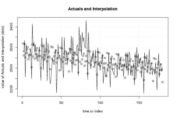Multiple Linear Regression - Actuals, Interpolation, and Residuals Time or Index Actuals Interpolation Forecast Residuals Prediction Error 1 2938 3078.47291666666 -140.472916666662 2 2909 2846.87291666667 62.1270833333328 3 3141 3065.67291666667 75.3270833333329 4 2427 2806.20625 -379.20625 5 3059 2891.13958333333 167.860416666666 6 2918 2963.40625 -45.4062500000003 7 2901 3006.07291666667 -105.072916666667 8 2823 2771.00625 51.99375 9 2798 2852.53958333333 -54.5395833333332 10 2892 2961.87291666667 -69.872916666667 11 2967 2859.47291666667 107.527083333333 12 2397 2618.93958333333 -221.939583333333 13 3458 3057.93869047619 400.061309523809 14 3024 2826.33869047619 197.661309523809 15 3100 3045.13869047619 54.8613095238095 16 2904 2785.67202380952 118.327976190476 17 3056 2870.60535714286 185.394642857143 18 2771 2942.87202380952 -171.872023809524 19 2897 2985.53869047619 -88.5386904761906 20 2772 2750.47202380952 21.5279761904761 21 2857 2832.00535714286 24.9946428571428 22 3020 2941.33869047619 78.6613095238096 23 2648 2838.93869047619 -190.938690476191 24 2364 2598.40535714286 -234.405357142857 25 3194 3037.40446428571 156.595535714285 26 3013 2805.80446428571 207.195535714286 27 2560 3024.60446428571 -464.604464285714 28 3074 2765.13779761905 308.862202380952 29 2746 2850.07113095238 -104.071130952381 30 2846 2922.33779761905 -76.3377976190476 31 3184 2965.00446428571 218.995535714286 32 2354 2729.93779761905 -375.937797619048 33 3080 2811.47113095238 268.528869047619 34 2963 2920.80446428571 42.1955357142857 35 2430 2818.40446428571 -388.404464285714 36 2296 2577.87113095238 -281.871130952381 37 2416 3016.87023809524 -600.870238095238 38 2647 2785.27023809524 -138.270238095238 39 2789 3004.07023809524 -215.070238095238 40 2685 2744.60357142857 -59.6035714285714 41 2666 2829.53690476190 -163.536904761905 42 2882 2901.80357142857 -19.8035714285715 43 2953 2944.47023809524 8.52976190476186 44 2127 2709.40357142857 -582.403571428572 45 2563 2790.93690476190 -227.936904761905 46 3061 2900.27023809524 160.729761904762 47 2809 2797.87023809524 11.1297619047618 48 2861 2557.33690476190 303.663095238095 49 2781 2996.33601190476 -215.336011904762 50 2555 2764.73601190476 -209.736011904762 51 3206 2983.53601190476 222.463988095238 52 2570 2724.06934523810 -154.069345238095 53 2410 2809.00267857143 -399.002678571429 54 3195 2881.26934523810 313.730654761905 55 2736 2923.93601190476 -187.936011904762 56 2743 2688.86934523810 54.1306547619047 57 2934 2770.40267857143 163.597321428571 58 2668 2879.73601190476 -211.736011904762 59 2907 2777.33601190476 129.663988095238 60 2866 2536.80267857143 329.197321428571 61 2983 2975.80178571429 7.19821428571394 62 2878 2744.20178571429 133.798214285714 63 3225 2963.00178571429 261.998214285714 64 2515 2703.53511904762 -188.535119047619 65 3193 2788.46845238095 404.531547619048 66 2663 2860.73511904762 -197.735119047619 67 2908 2903.40178571429 4.59821428571424 68 2896 2668.33511904762 227.664880952381 69 2853 2749.86845238095 103.131547619048 70 3028 2859.20178571429 168.798214285714 71 3053 2756.80178571429 296.198214285714 72 2455 2516.26845238095 -61.2684523809523 73 3401 2955.26755952381 445.73244047619 74 2969 2723.66755952381 245.332440476190 75 3243 2942.46755952381 300.532440476190 76 2849 2683.00089285714 165.999107142857 77 3296 2767.93422619048 528.065773809524 78 3121 2840.20089285714 280.799107142857 79 3194 2882.86755952381 311.132440476190 80 3023 2647.80089285714 375.199107142857 81 2984 2729.33422619048 254.665773809524 82 3525 2838.66755952381 686.33244047619 83 3116 2736.26755952381 379.732440476191 84 2383 2495.73422619048 -112.734226190476 85 3294 2934.73333333333 359.266666666666 86 2882 2703.13333333333 178.866666666667 87 2820 2921.93333333333 -101.933333333333 88 2583 2662.46666666667 -79.4666666666667 89 2803 2747.4 55.6 90 2767 2819.66666666667 -52.6666666666666 91 2945 2862.33333333333 82.6666666666667 92 2716 2627.26666666667 88.7333333333333 93 2644 2708.8 -64.8 94 2956 2818.13333333333 137.866666666667 95 2598 2715.73333333333 -117.733333333333 96 2171 2475.2 -304.2 97 2994 2914.19910714286 79.8008928571425 98 2645 2682.59910714286 -37.5991071428571 99 2724 2901.39910714286 -177.399107142857 100 2550 2641.93244047619 -91.9324404761905 101 2707 2726.86577380952 -19.8657738095238 102 2679 2799.13244047619 -120.132440476190 103 2878 2841.79910714286 36.2008928571428 104 2307 2606.73244047619 -299.732440476190 105 2496 2688.26577380952 -192.265773809524 106 2637 2797.59910714286 -160.599107142857 107 2436 2695.19910714286 -259.199107142857 108 2426 2454.66577380952 -28.6657738095237 109 2607 2893.66488095238 -286.664880952381 110 2533 2662.06488095238 -129.064880952381 111 2888 2880.86488095238 7.13511904761912 112 2520 2621.39821428571 -101.398214285714 113 2229 2706.33154761905 -477.331547619048 114 2804 2778.59821428571 25.4017857142858 115 2661 2821.26488095238 -160.264880952381 116 2547 2586.19821428571 -39.1982142857143 117 2509 2667.73154761905 -158.731547619048 118 2465 2777.06488095238 -312.064880952381 119 2629 2674.66488095238 -45.664880952381 120 2706 2434.13154761905 271.868452380952 121 2666 2873.13065476191 -207.130654761905 122 2432 2641.53065476190 -209.530654761905 123 2836 2860.33065476190 -24.3306547619047 124 2888 2600.86398809524 287.136011904762 125 2566 2685.79732142857 -119.797321428571 126 2802 2758.06398809524 43.936011904762 127 2611 2800.73065476190 -189.730654761905 128 2683 2565.66398809524 117.336011904762 129 2675 2647.19732142857 27.8026785714286 130 2434 2756.53065476190 -322.530654761905 131 2693 2654.13065476190 38.8693452380953 132 2619 2413.59732142857 205.402678571429 133 2903 2852.59642857143 50.4035714285711 134 2550 2620.99642857143 -70.9964285714285 135 2900 2839.79642857143 60.2035714285715 136 2456 2580.32976190476 -124.329761904762 137 2912 2665.26309523810 246.736904761905 138 2883 2737.52976190476 145.470238095238 139 2464 2780.19642857143 -316.196428571429 140 2655 2545.12976190476 109.870238095238 141 2447 2626.66309523810 -179.663095238095 142 2592 2735.99642857143 -143.996428571428 143 2698 2633.59642857143 64.4035714285715 144 2274 2393.06309523810 -119.063095238095 145 2901 2832.06220238095 68.9377976190474 146 2397 2600.46220238095 -203.462202380952 147 3004 2819.26220238095 184.737797619048 148 2614 2559.79553571429 54.2044642857144 149 2882 2644.72886904762 237.271130952381 150 2671 2716.99553571429 -45.9955357142857 151 2761 2759.66220238095 1.33779761904765 152 2806 2524.59553571429 281.404464285714 153 2414 2606.12886904762 -192.128869047619 154 2673 2715.46220238095 -42.4622023809523 155 2748 2613.06220238095 134.937797619048 156 2112 2372.52886904762 -260.528869047619 157 2903 2811.52797619048 91.4720238095235 158 2633 2579.92797619048 53.0720238095239 159 2684 2798.72797619048 -114.727976190476 160 2861 2539.26130952381 321.738690476191 161 2504 2624.19464285714 -120.194642857143 162 2708 2696.46130952381 11.5386904761906 163 2961 2739.12797619048 221.872023809524 164 2535 2504.06130952381 30.9386904761905 165 2688 2585.59464285714 102.405357142857 166 2699 2694.92797619048 4.07202380952389 167 2469 2592.52797619048 -123.527976190476 168 2585 2351.99464285714 233.005357142857 169 2582 2790.99375 -208.993750000000 170 2480 2559.39375 -79.3937499999999 171 2709 2778.19375 -69.1937499999999 172 2441 2518.72708333333 -77.7270833333332 173 2182 2603.66041666667 -421.660416666667 174 2585 2675.92708333333 -90.9270833333333 175 2881 2718.59375 162.40625 176 2422 2483.52708333333 -61.5270833333333 177 2690 2565.06041666667 124.939583333333 178 2659 2674.39375 -15.3937499999999 179 2535 2571.99375 -36.99375 180 2613 2331.46041666667 281.539583333333 Goldfeld-Quandt test for Heteroskedasticity p-values Alternative Hypothesis breakpoint index greater 2-sided less 16 0.471113114851855 0.94222622970371 0.528886885148145 17 0.406722254768837 0.813444509537675 0.593277745231163 18 0.427823128339037 0.855646256678074 0.572176871660963 19 0.328724225384515 0.65744845076903 0.671275774615485 20 0.255871197815032 0.511742395630064 0.744128802184968 21 0.171940437658687 0.343880875317373 0.828059562341313 22 0.109788007253362 0.219576014506725 0.890211992746638 23 0.173158025457279 0.346316050914557 0.826841974542721 24 0.125261087218309 0.250522174436618 0.874738912781691 25 0.0874444163239566 0.174888832647913 0.912555583676043 26 0.0575143480300309 0.115028696060062 0.94248565196997 27 0.28055402759019 0.56110805518038 0.71944597240981 28 0.376691600258199 0.753383200516399 0.623308399741801 29 0.400301677700772 0.800603355401543 0.599698322299228 30 0.329846393903087 0.659692787806174 0.670153606096913 31 0.334487206098252 0.668974412196504 0.665512793901748 32 0.45381690246158 0.90763380492316 0.54618309753842 33 0.452208328679755 0.90441665735951 0.547791671320245 34 0.385375357052996 0.770750714105992 0.614624642947004 35 0.454292908843279 0.908585817686558 0.545707091156721 36 0.413624107714939 0.827248215429878 0.586375892285061 37 0.783773488520543 0.432453022958914 0.216226511479457 38 0.762739424504448 0.474521150991103 0.237260575495552 39 0.728831973399385 0.542336053201229 0.271168026600615 40 0.679072374017546 0.641855251964907 0.320927625982454 41 0.645572220921196 0.708855558157608 0.354427779078804 42 0.613486430822626 0.773027138354749 0.386513569177375 43 0.563009303213906 0.873981393572187 0.436990696786094 44 0.711364043908718 0.577271912182565 0.288635956091282 45 0.701589421564555 0.59682115687089 0.298410578435445 46 0.695403252424391 0.609193495151219 0.304596747575609 47 0.691320915604289 0.617358168791423 0.308679084395711 48 0.838022279750906 0.323955440498188 0.161977720249094 49 0.824010818257052 0.351978363485895 0.175989181742948 50 0.817446652870372 0.365106694259257 0.182553347129628 51 0.858453163302827 0.283093673394347 0.141546836697173 52 0.839699806540674 0.320600386918652 0.160300193459326 53 0.886953677606455 0.226092644787089 0.113046322393544 54 0.922819212727609 0.154361574544782 0.077180787272391 55 0.916545700715933 0.166908598568134 0.083454299284067 56 0.921820577940353 0.156358844119295 0.0781794220596473 57 0.912511724814784 0.174976550370433 0.0874882751852163 58 0.913513524030644 0.172972951938712 0.0864864759693562 59 0.910917949619232 0.178164100761536 0.0890820503807679 60 0.93673630603894 0.126527387922119 0.0632636939610596 61 0.924104723860933 0.151790552278134 0.075895276139067 62 0.909311860602005 0.181376278795989 0.0906881393979945 63 0.91480683270804 0.170386334583921 0.0851931672919604 64 0.913091558003433 0.173816883993134 0.0869084419965668 65 0.942344000997874 0.115311998004252 0.0576559990021262 66 0.943574949104955 0.112850101790091 0.0564250508950455 67 0.930122650872807 0.139754698254386 0.0698773491271932 68 0.935194415110818 0.129611169778363 0.0648055848891815 69 0.91950503578316 0.160989928433678 0.0804949642168391 70 0.905625754720529 0.188748490558943 0.0943742452794714 71 0.911115427522478 0.177769144955043 0.0888845724775216 72 0.896371014955676 0.207257970088647 0.103628985044324 73 0.93223953380204 0.135520932395922 0.0677604661979608 74 0.926698935649124 0.146602128701753 0.0733010643508764 75 0.928213233715492 0.143573532569016 0.0717867662845078 76 0.915239022536406 0.169521954927187 0.0847609774635935 77 0.959966436728253 0.080067126543495 0.0400335632717475 78 0.959736435533308 0.0805271289333834 0.0402635644666917 79 0.962665976231223 0.074668047537555 0.0373340237687775 80 0.971628301065793 0.0567433978684144 0.0283716989342072 81 0.972216806394315 0.0555663872113701 0.0277831936056850 82 0.997984434089737 0.00403113182052672 0.00201556591026336 83 0.999084612726846 0.00183077454630845 0.000915387273154224 84 0.998921951336664 0.00215609732667142 0.00107804866333571 85 0.99953215318233 0.000935693635338657 0.000467846817669329 86 0.999637341510814 0.000725316978372753 0.000362658489186376 87 0.999591530958219 0.000816938083562786 0.000408469041781393 88 0.99947458411162 0.00105083177675827 0.000525415888379134 89 0.99946035438104 0.00107929123791976 0.00053964561895988 90 0.999293640834564 0.00141271833087145 0.000706359165435723 91 0.999162595131518 0.0016748097369643 0.00083740486848215 92 0.998905257153716 0.00218948569256851 0.00109474284628425 93 0.998743572944987 0.00251285411002513 0.00125642705501256 94 0.999198602941353 0.00160279411729395 0.000801397058646976 95 0.999052605202675 0.00189478959464964 0.000947394797324819 96 0.999441269250991 0.00111746149801723 0.000558730749008617 97 0.999431242151243 0.00113751569751389 0.000568757848756944 98 0.99936670249405 0.00126659501189889 0.000633297505949446 99 0.99929193968898 0.00141612062204026 0.00070806031102013 100 0.999034687763582 0.00193062447283611 0.000965312236418057 101 0.998920407366753 0.00215918526649379 0.00107959263324690 102 0.998583772671743 0.00283245465651409 0.00141622732825705 103 0.99828555340058 0.00342889319883957 0.00171444659941978 104 0.998872488027914 0.00225502394417138 0.00112751197208569 105 0.998701094709022 0.00259781058195689 0.00129890529097844 106 0.9985372944373 0.00292541112539806 0.00146270556269903 107 0.998636824132312 0.0027263517353754 0.0013631758676877 108 0.998025209739897 0.00394958052020617 0.00197479026010308 109 0.998268752448119 0.00346249510376305 0.00173124755188152 110 0.997717487729171 0.00456502454165771 0.00228251227082885 111 0.99672123217435 0.00655753565129955 0.00327876782564978 112 0.99583438379029 0.00833123241941908 0.00416561620970954 113 0.998751797517073 0.00249640496585367 0.00124820248292684 114 0.998146593884327 0.00370681223134635 0.00185340611567317 115 0.997606266786172 0.00478746642765556 0.00239373321382778 116 0.996712055856209 0.00657588828758232 0.00328794414379116 117 0.995828445395037 0.00834310920992669 0.00417155460496334 118 0.996270719774528 0.00745856045094384 0.00372928022547192 119 0.994661026326684 0.0106779473466327 0.00533897367331633 120 0.995046133619124 0.00990773276175124 0.00495386638087562 121 0.99466761056363 0.0106647788727389 0.00533238943636943 122 0.993593709255923 0.0128125814881548 0.0064062907440774 123 0.99083897185904 0.0183220562819203 0.00916102814096015 124 0.992006854577691 0.015986290844618 0.007993145422309 125 0.989344663809746 0.0213106723805080 0.0106553361902540 126 0.985072344898303 0.0298553102033946 0.0149276551016973 127 0.98389472401774 0.0322105519645207 0.0161052759822603 128 0.978217446570073 0.0435651068598539 0.0217825534299270 129 0.970475303514675 0.059049392970649 0.0295246964853245 130 0.976055144780082 0.0478897104398363 0.0239448552199181 131 0.966962422446486 0.0660751551070286 0.0330375775535143 132 0.962364063442283 0.0752718731154338 0.0376359365577169 133 0.949941394985902 0.100117210028197 0.0500586050140984 134 0.933482816849873 0.133034366300255 0.0665171831501274 135 0.913928271991283 0.172143456017434 0.0860717280087172 136 0.90767745913574 0.184645081728520 0.0923225408642601 137 0.928546410626313 0.142907178747374 0.0714535893736869 138 0.921775188151205 0.156449623697590 0.0782248118487948 139 0.95927238951813 0.0814552209637408 0.0407276104818704 140 0.944315072318358 0.111369855363283 0.0556849276816416 141 0.939004392252862 0.121991215494275 0.0609956077471376 142 0.926567605623128 0.146864788753744 0.0734323943768718 143 0.901559410947455 0.196881178105089 0.0984405890525447 144 0.90043973795007 0.199120524099859 0.0995602620499295 145 0.871007447350643 0.257985105298713 0.128992552649357 146 0.86545437993717 0.269091240125658 0.134545620062829 147 0.85719509904288 0.285609801914241 0.142804900957120 148 0.820647619921942 0.358704760156117 0.179352380078058 149 0.914119420186618 0.171761159626765 0.0858805798133825 150 0.879530745697454 0.240938508605092 0.120469254302546 151 0.864423112849418 0.271153774301163 0.135576887150582 152 0.879152044080873 0.241695911838253 0.120847955919127 153 0.905208317515966 0.189583364968068 0.094791682484034 154 0.86704286260255 0.265914274794900 0.132957137397450 155 0.842302897717944 0.315394204564112 0.157697102282056 156 0.994474732336028 0.0110505353279442 0.00552526766397211 157 0.994090724189603 0.0118185516207936 0.0059092758103968 158 0.987387006880817 0.0252259862383658 0.0126129931191829 159 0.978964257245377 0.0420714855092466 0.0210357427546233 160 0.99480540125336 0.0103891974932801 0.00519459874664007 161 0.999458859900868 0.00108228019826311 0.000541140099131556 162 0.998830923203843 0.00233815359231398 0.00116907679615699 163 0.995981929182622 0.00803614163475582 0.00401807081737791 164 0.996290138681728 0.00741972263654331 0.00370986131827166 Meta Analysis of Goldfeld-Quandt test for Heteroskedasticity Description # significant tests % significant tests OK/NOK 1% type I error level 42 0.281879194630872 NOK 5% type I error level 57 0.38255033557047 NOK 10% type I error level 66 0.442953020134228 NOK

Charts produced by software:

http://www.freestatistics.org/blog/date/2010/Nov/30/t1291114182lynqj1vuqelvg67/10iub41291114246.png (open in new window) http://www.freestatistics.org/blog/date/2010/Nov/30/t1291114182lynqj1vuqelvg67/10iub41291114246.ps (open in new window) http://www.freestatistics.org/blog/date/2010/Nov/30/t1291114182lynqj1vuqelvg67/1m2dv1291114246.png (open in new window) http://www.freestatistics.org/blog/date/2010/Nov/30/t1291114182lynqj1vuqelvg67/1m2dv1291114246.ps (open in new window) http://www.freestatistics.org/blog/date/2010/Nov/30/t1291114182lynqj1vuqelvg67/2m2dv1291114246.png (open in new window) http://www.freestatistics.org/blog/date/2010/Nov/30/t1291114182lynqj1vuqelvg67/2m2dv1291114246.ps (open in new window) http://www.freestatistics.org/blog/date/2010/Nov/30/t1291114182lynqj1vuqelvg67/3fbcg1291114246.png (open in new window) http://www.freestatistics.org/blog/date/2010/Nov/30/t1291114182lynqj1vuqelvg67/3fbcg1291114246.ps (open in new window) http://www.freestatistics.org/blog/date/2010/Nov/30/t1291114182lynqj1vuqelvg67/4fbcg1291114246.png (open in new window) http://www.freestatistics.org/blog/date/2010/Nov/30/t1291114182lynqj1vuqelvg67/4fbcg1291114246.ps (open in new window) http://www.freestatistics.org/blog/date/2010/Nov/30/t1291114182lynqj1vuqelvg67/5fbcg1291114246.png (open in new window) http://www.freestatistics.org/blog/date/2010/Nov/30/t1291114182lynqj1vuqelvg67/5fbcg1291114246.ps (open in new window) http://www.freestatistics.org/blog/date/2010/Nov/30/t1291114182lynqj1vuqelvg67/68kuj1291114246.png (open in new window) http://www.freestatistics.org/blog/date/2010/Nov/30/t1291114182lynqj1vuqelvg67/68kuj1291114246.ps (open in new window) http://www.freestatistics.org/blog/date/2010/Nov/30/t1291114182lynqj1vuqelvg67/78kuj1291114246.png (open in new window) http://www.freestatistics.org/blog/date/2010/Nov/30/t1291114182lynqj1vuqelvg67/78kuj1291114246.ps (open in new window) http://www.freestatistics.org/blog/date/2010/Nov/30/t1291114182lynqj1vuqelvg67/8iub41291114246.png (open in new window) http://www.freestatistics.org/blog/date/2010/Nov/30/t1291114182lynqj1vuqelvg67/8iub41291114246.ps (open in new window) http://www.freestatistics.org/blog/date/2010/Nov/30/t1291114182lynqj1vuqelvg67/9iub41291114246.png (open in new window) http://www.freestatistics.org/blog/date/2010/Nov/30/t1291114182lynqj1vuqelvg67/9iub41291114246.ps (open in new window)

Parameters (Session):

par1 = 1 ; par2 = Include Monthly Dummies ; par3 = Linear Trend ;

Parameters (R input):

par1 = 1 ; par2 = Include Monthly Dummies ; par3 = Linear Trend ;

R code (references can be found in the software module):

library(lattice) library(lmtest) n25 <- 25 #minimum number of obs. for Goldfeld-Quandt test par1 <- as.numeric(par1) x <- t(y) k <- length(x[1,]) n <- length(x[,1]) x1 <- cbind(x[,par1], x[,1:k!=par1]) mycolnames <- c(colnames(x)[par1], colnames(x)[1:k!=par1]) colnames(x1) <- mycolnames #colnames(x)[par1] x <- x1 if (par3 == 'First Differences'){ x2 <- array(0, dim=c(n-1,k), dimnames=list(1:(n-1), paste('(1-B)',colnames(x),sep=''))) for (i in 1:n-1) { for (j in 1:k) { x2[i,j] <- x[i+1,j] - x[i,j] } } x <- x2 } if (par2 == 'Include Monthly Dummies'){ x2 <- array(0, dim=c(n,11), dimnames=list(1:n, paste('M', seq(1:11), sep =''))) for (i in 1:11){ x2[seq(i,n,12),i] <- 1 } x <- cbind(x, x2) } if (par2 == 'Include Quarterly Dummies'){ x2 <- array(0, dim=c(n,3), dimnames=list(1:n, paste('Q', seq(1:3), sep =''))) for (i in 1:3){ x2[seq(i,n,4),i] <- 1 } x <- cbind(x, x2) } k <- length(x[1,]) if (par3 == 'Linear Trend'){ x <- cbind(x, c(1:n)) colnames(x)[k+1] <- 't' } x k <- length(x[1,]) df <- as.data.frame(x) (mylm <- lm(df)) (mysum <- summary(mylm)) if (n > n25) { kp3 <- k + 3 nmkm3 <- n - k - 3 gqarr <- array(NA, dim=c(nmkm3-kp3+1,3)) numgqtests <- 0 numsignificant1 <- 0 numsignificant5 <- 0 numsignificant10 <- 0 for (mypoint in kp3:nmkm3) { j <- 0 numgqtests <- numgqtests + 1 for (myalt in c('greater', 'two.sided', 'less')) { j <- j + 1 gqarr[mypoint-kp3+1,j] <- gqtest(mylm, point=mypoint, alternative=myalt)$p.value } if (gqarr[mypoint-kp3+1,2] < 0.01) numsignificant1 <- numsignificant1 + 1 if (gqarr[mypoint-kp3+1,2] < 0.05) numsignificant5 <- numsignificant5 + 1 if (gqarr[mypoint-kp3+1,2] < 0.10) numsignificant10 <- numsignificant10 + 1 } gqarr } bitmap(file='test0.png') plot(x[,1], type='l', main='Actuals and Interpolation', ylab='value of Actuals and Interpolation (dots)', xlab='time or index') points(x[,1]-mysum$resid) grid() dev.off() bitmap(file='test1.png') plot(mysum$resid, type='b', pch=19, main='Residuals', ylab='value of Residuals', xlab='time or index') grid() dev.off() bitmap(file='test2.png') hist(mysum$resid, main='Residual Histogram', xlab='values of Residuals') grid() dev.off() bitmap(file='test3.png') densityplot(~mysum$resid,col='black',main='Residual Density Plot', xlab='values of Residuals') dev.off() bitmap(file='test4.png') 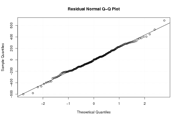qqnorm(mysum$resid, main='Residual Normal Q-Q Plot') qqline(mysum$resid) grid() dev.off() (myerror <- as.ts(mysum$resid)) 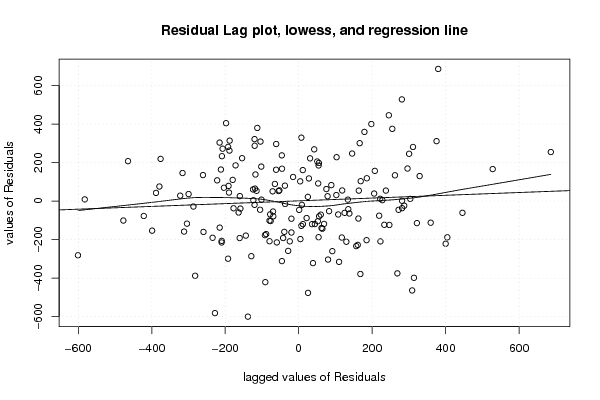bitmap(file='test5.png') dum <- cbind(lag(myerror,k=1),myerror) dum dum1 <- dum[2:length(myerror),] dum1 z <- as.data.frame(dum1) z plot(z,main=paste('Residual Lag plot, lowess, and regression line'), ylab='values of Residuals', xlab='lagged values of Residuals') lines(lowess(z)) abline(lm(z)) grid() dev.off() bitmap(file='test6.png') 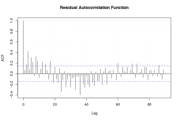acf(mysum$resid, lag.max=length(mysum$resid)/2, main='Residual Autocorrelation Function') grid() dev.off() bitmap(file='test7.png') pacf(mysum$resid, lag.max=length(mysum$resid)/2, main='Residual Partial Autocorrelation Function') grid() dev.off() bitmap(file='test8.png') 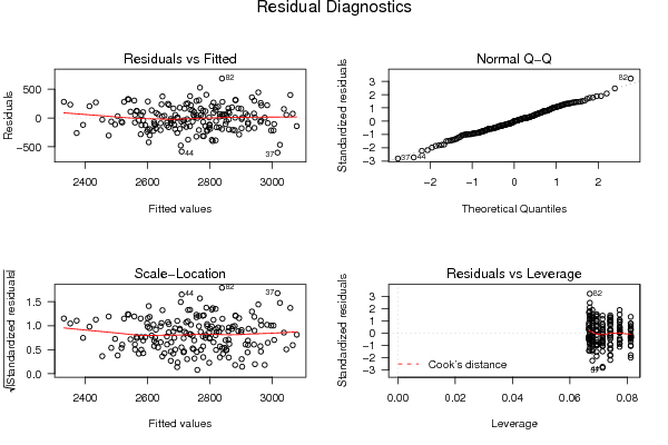opar <- par(mfrow = c(2,2), oma = c(0, 0, 1.1, 0)) plot(mylm, las = 1, sub='Residual Diagnostics') par(opar) dev.off() if (n > n25) { bitmap(file='test9.png') plot(kp3:nmkm3,gqarr[,2], main='Goldfeld-Quandt test',ylab='2-sided p-value',xlab='breakpoint') grid() dev.off() } load(file='createtable') a<-table.start() a<-table.row.start(a) a<-table.element(a, 'Multiple Linear Regression - Estimated Regression Equation', 1, TRUE) a<-table.row.end(a) myeq <- colnames(x)[1] myeq <- paste(myeq, '[t] = ', sep='') for (i in 1:k){ if (mysum$coefficients[i,1] > 0) myeq <- paste(myeq, '+', '') myeq <- paste(myeq, mysum$coefficients[i,1], sep=' ') if (rownames(mysum$coefficients)[i] != '(Intercept)') { myeq <- paste(myeq, rownames(mysum$coefficients)[i], sep='') if (rownames(mysum$coefficients)[i] != 't') myeq <- paste(myeq, '[t]', sep='') } } myeq <- paste(myeq, ' + e[t]') a<-table.row.start(a) a<-table.element(a, myeq) a<-table.row.end(a) a<-table.end(a) table.save(a,file='mytable1.tab') a<-table.start() a<-table.row.start(a) a<-table.element(a,hyperlink('http://www.xycoon.com/ols1.htm','Multiple Linear Regression - Ordinary Least Squares',''), 6, TRUE) a<-table.row.end(a) a<-table.row.start(a) a<-table.element(a,'Variable',header=TRUE) a<-table.element(a,'Parameter',header=TRUE) a<-table.element(a,'S.D.',header=TRUE) a<-table.element(a,'T-STAT<br />H0: parameter = 0',header=TRUE) a<-table.element(a,'2-tail p-value',header=TRUE) a<-table.element(a,'1-tail p-value',header=TRUE) a<-table.row.end(a) for (i in 1:k){ a<-table.row.start(a) a<-table.element(a,rownames(mysum$coefficients)[i],header=TRUE) a<-table.element(a,mysum$coefficients[i,1]) a<-table.element(a, round(mysum$coefficients[i,2],6)) a<-table.element(a, round(mysum$coefficients[i,3],4)) a<-table.element(a, round(mysum$coefficients[i,4],6)) a<-table.element(a, round(mysum$coefficients[i,4]/2,6)) a<-table.row.end(a) } a<-table.end(a) table.save(a,file='mytable2.tab') a<-table.start() a<-table.row.start(a) a<-table.element(a, 'Multiple Linear Regression - Regression Statistics', 2, TRUE) a<-table.row.end(a) a<-table.row.start(a) a<-table.element(a, 'Multiple R',1,TRUE) a<-table.element(a, sqrt(mysum$r.squared)) a<-table.row.end(a) a<-table.row.start(a) a<-table.element(a, 'R-squared',1,TRUE) a<-table.element(a, mysum$r.squared) a<-table.row.end(a) a<-table.row.start(a) a<-table.element(a, 'Adjusted R-squared',1,TRUE) a<-table.element(a, mysum$adj.r.squared) a<-table.row.end(a) a<-table.row.start(a) a<-table.element(a, 'F-TEST (value)',1,TRUE) a<-table.element(a, mysum$fstatistic[1]) a<-table.row.end(a) a<-table.row.start(a) a<-table.element(a, 'F-TEST (DF numerator)',1,TRUE) a<-table.element(a, mysum$fstatistic[2]) a<-table.row.end(a) a<-table.row.start(a) a<-table.element(a, 'F-TEST (DF denominator)',1,TRUE) a<-table.element(a, mysum$fstatistic[3]) a<-table.row.end(a) a<-table.row.start(a) a<-table.element(a, 'p-value',1,TRUE) a<-table.element(a, 1-pf(mysum$fstatistic[1],mysum$fstatistic[2],mysum$fstatistic[3])) a<-table.row.end(a) a<-table.row.start(a) a<-table.element(a, 'Multiple Linear Regression - Residual Statistics', 2, TRUE) a<-table.row.end(a) a<-table.row.start(a) a<-table.element(a, 'Residual Standard Deviation',1,TRUE) a<-table.element(a, mysum$sigma) a<-table.row.end(a) a<-table.row.start(a) a<-table.element(a, 'Sum Squared Residuals',1,TRUE) a<-table.element(a, sum(myerror*myerror)) a<-table.row.end(a) a<-table.end(a) table.save(a,file='mytable3.tab') a<-table.start() a<-table.row.start(a) a<-table.element(a, 'Multiple Linear Regression - Actuals, Interpolation, and Residuals', 4, TRUE) a<-table.row.end(a) a<-table.row.start(a) a<-table.element(a, 'Time or Index', 1, TRUE) a<-table.element(a, 'Actuals', 1, TRUE) a<-table.element(a, 'Interpolation<br />Forecast', 1, TRUE) a<-table.element(a, 'Residuals<br />Prediction Error', 1, TRUE) a<-table.row.end(a) for (i in 1:n) { a<-table.row.start(a) a<-table.element(a,i, 1, TRUE) a<-table.element(a,x[i]) a<-table.element(a,x[i]-mysum$resid[i]) a<-table.element(a,mysum$resid[i]) a<-table.row.end(a) } a<-table.end(a) table.save(a,file='mytable4.tab') if (n > n25) { a<-table.start() a<-table.row.start(a) a<-table.element(a,'Goldfeld-Quandt test for Heteroskedasticity',4,TRUE) a<-table.row.end(a) a<-table.row.start(a) a<-table.element(a,'p-values',header=TRUE) a<-table.element(a,'Alternative Hypothesis',3,header=TRUE) a<-table.row.end(a) a<-table.row.start(a) a<-table.element(a,'breakpoint index',header=TRUE) a<-table.element(a,'greater',header=TRUE) a<-table.element(a,'2-sided',header=TRUE) a<-table.element(a,'less',header=TRUE) a<-table.row.end(a) for (mypoint in kp3:nmkm3) { a<-table.row.start(a) a<-table.element(a,mypoint,header=TRUE) a<-table.element(a,gqarr[mypoint-kp3+1,1]) a<-table.element(a,gqarr[mypoint-kp3+1,2]) a<-table.element(a,gqarr[mypoint-kp3+1,3]) a<-table.row.end(a) } a<-table.end(a) table.save(a,file='mytable5.tab') a<-table.start() a<-table.row.start(a) a<-table.element(a,'Meta Analysis of Goldfeld-Quandt test for Heteroskedasticity',4,TRUE) a<-table.row.end(a) a<-table.row.start(a) a<-table.element(a,'Description',header=TRUE) a<-table.element(a,'# significant tests',header=TRUE) a<-table.element(a,'% significant tests',header=TRUE) a<-table.element(a,'OK/NOK',header=TRUE) a<-table.row.end(a) a<-table.row.start(a) a<-table.element(a,'1% type I error level',header=TRUE) a<-table.element(a,numsignificant1) a<-table.element(a,numsignificant1/numgqtests) if (numsignificant1/numgqtests < 0.01) dum <- 'OK' else dum <- 'NOK' a<-table.element(a,dum) a<-table.row.end(a) a<-table.row.start(a) a<-table.element(a,'5% type I error level',header=TRUE) a<-table.element(a,numsignificant5) a<-table.element(a,numsignificant5/numgqtests) if (numsignificant5/numgqtests < 0.05) dum <- 'OK' else dum <- 'NOK' a<-table.element(a,dum) a<-table.row.end(a) a<-table.row.start(a) a<-table.element(a,'10% type I error level',header=TRUE) a<-table.element(a,numsignificant10) a<-table.element(a,numsignificant10/numgqtests) if (numsignificant10/numgqtests < 0.1) dum <- 'OK' else dum <- 'NOK' a<-table.element(a,dum) a<-table.row.end(a) a<-table.end(a) table.save(a,file='mytable6.tab') }

Copyright

This work is licensed under a Creative Commons Attribution-Noncommercial-Share Alike 3.0 License.

Software written by Ed van Stee & Patrick Wessa

Disclaimer

Information provided on this web site is provided "AS IS" without warranty of any kind, either express or implied, including, without limitation, warranties of merchantability, fitness for a particular purpose, and noninfringement. We use reasonable efforts to include accurate and timely information and periodically update the information, and software without notice. However, we make no warranties or representations as to the accuracy or completeness of such information (or software), and we assume no liability or responsibility for errors or omissions in the content of this web site, or any software bugs in online applications. Your use of this web site is AT YOUR OWN RISK. Under no circumstances and under no legal theory shall we be liable to you or any other person for any direct, indirect, special, incidental, exemplary, or consequential damages arising from your access to, or use of, this web site.

Privacy Policy

We may request personal information to be submitted to our servers in order to be able to:

• personalize online software applications according to your needs
• enforce strict security rules with respect to the data that you upload (e.g. statistical data)
• manage user sessions of online applications
• alert you about important changes or upgrades in resources or applications

We NEVER allow other companies to directly offer registered users information about their products and services. Banner references and hyperlinks of third parties NEVER contain any personal data of the visitor.

We do NOT sell, nor transmit by any means, personal information, nor statistical data series uploaded by you to third parties.

We carefully protect your data from loss, misuse, alteration, and destruction. However, at any time, and under any circumstance you are solely responsible for managing your passwords, and keeping them secret.

We store a unique ANONYMOUS USER ID in the form of a small 'Cookie' on your computer. This allows us to track your progress when using this website which is necessary to create state-dependent features. The cookie is used for NO OTHER PURPOSE. At any time you may opt to disallow cookies from this website - this will not affect other features of this website.

We examine cookies that are used by third-parties (banner and online ads) very closely: abuse from third-parties automatically results in termination of the advertising contract without refund. We have very good reason to believe that the cookies that are produced by third parties (banner ads) do NOT cause any privacy or security risk.

FreeStatistics.org is safe. There is no need to download any software to use the applications and services contained in this website. Hence, your system's security is not compromised by their use, and your personal data - other than data you submit in the account application form, and the user-agent information that is transmitted by your browser - is never transmitted to our servers.

As a general rule, we do not log on-line behavior of individuals (other than normal logging of webserver 'hits'). However, in cases of abuse, hacking, unauthorized access, Denial of Service attacks, illegal copying, hotlinking, non-compliance with international webstandards (such as robots.txt), or any other harmful behavior, our system engineers are empowered to log, track, identify, publish, and ban misbehaving individuals - even if this leads to ban entire blocks of IP addresses, or disclosing user's identity.

FreeStatistics.org is powered by