mini tutorial multiple linear regression

*The author of this computation has been verified*

R Software Module: /rwasp_multipleregression.wasp (opens new window with default values)

Title produced by software: Multiple Regression

Date of computation: Tue, 30 Nov 2010 13:02:25 +0000

Cite this page as follows:

Statistical Computations at FreeStatistics.org, Office for Research Development and Education, URL http://www.freestatistics.org/blog/date/2010/Nov/30/t1291122381039j728zuhw8wg8.htm/, Retrieved Tue, 30 Nov 2010 14:06:32 +0100

BibTeX entries for LaTeX users:

@Manual{KEY, author = {{YOUR NAME}}, publisher = {Office for Research Development and Education}, title = {Statistical Computations at FreeStatistics.org, URL http://www.freestatistics.org/blog/date/2010/Nov/30/t1291122381039j728zuhw8wg8.htm/}, year = {2010}, } @Manual{R, title = {R: A Language and Environment for Statistical Computing}, author = {{R Development Core Team}}, organization = {R Foundation for Statistical Computing}, address = {Vienna, Austria}, year = {2010}, note = {{ISBN} 3-900051-07-0}, url = {http://www.R-project.org}, }

Original text written by user:

IsPrivate?

No (this computation is public)

User-defined keywords:

Dataseries X:

» Textbox « » Textfile « » CSV «

2284 33 41 76403 194493 3160 108 90 108094 530670 4150 150 136 134759 518365 7285 115 97 188873 491303 1134 162 63 146216 527021 4658 158 114 156608 233773 2384 97 77 61348 405972 3748 9 6 50350 652925 5371 66 47 87720 446211 1285 107 51 99489 341340 9327 101 85 87419 387699 5565 47 43 94355 493408 1528 38 32 60326 146494 3122 34 25 94670 414462 7561 87 77 82425 364304 2675 79 54 59017 355178 13253 947 251 90829 357760 880 74 15 80791 261216 2053 53 44 100423 397144 1424 94 73 131116 374943 4036 63 85 100269 424898 3045 58 49 27330 202055 5119 49 38 39039 378525 1431 34 35 106885 310768 554 11 9 79285 325738 1975 35 34 118881 394510 1765 20 20 77623 247060 1012 47 29 114768 368078 810 43 11 74015 236761 1280 117 52 69465 312378 666 171 13 117869 339836 1380 26 29 60982 347385 4677 75 66 90131 426280 876 59 33 138971 352850 814 18 15 39625 301881 514 15 15 102725 377516 5692 72 68 64239 357312 3642 86 100 90262 458343 540 14 13 103960 354228 2099 64 45 106611 308636 567 etc...

Output produced by software:

Enter (or paste) a matrix (table) containing all data (time) series. Every column represents a different variable and must be delimited by a space or Tab. Every row represents a period in time (or category) and must be delimited by hard returns. The easiest way to enter data is to copy and paste a block of spreadsheet cells. Please, do not use commas or spaces to seperate groups of digits! Summary of computational transaction Raw Input view raw input (R code) Raw Output view raw output of R engine Computing time 6 seconds R Server 'Gwilym Jenkins' @ 72.249.127.135 Multiple Linear Regression - Estimated Regression Equation Wealth[t] = + 277356.379214211 + 9.68627414559874Costs[t] -215.764818638136Trades[t] + 397.451574439388Orders[t] + 0.693364216186951Dividends[t] + e[t] Multiple Linear Regression - Ordinary Least Squares Variable Parameter S.D. T-STAT H0: parameter = 0 2-tail p-value 1-tail p-value (Intercept) 277356.379214211 39187.296117 7.0777 0 0 Costs 9.68627414559874 7.267258 1.3329 0.18914 0.09457 Trades -215.764818638136 158.358849 -1.3625 0.179672 0.089836 Orders 397.451574439388 599.73889 0.6627 0.510825 0.255412 Dividends 0.693364216186951 0.400191 1.7326 0.08987 0.044935 Multiple Linear Regression - Regression Statistics Multiple R 0.392827243240654 R-squared 0.154313243032052 Adjusted R-squared 0.080775264165274 F-TEST (value) 2.09841561340171 F-TEST (DF numerator) 4 F-TEST (DF denominator) 46 p-value 0.0963284682016443 Multiple Linear Regression - Residual Statistics Residual Standard Deviation 87541.7774609282 Sum Squared Residuals 352523888846.859 Multiple Linear Regression - Actuals, Interpolation, and Residuals Time or Index Actuals Interpolation Forecast Residuals Prediction Error 1 194493 361630.211109046 -167137.211109046 2 530670 395381.558385441 135288.441614559 3 518365 432680.176655619 85684.8233443808 4 491303 492618.514546011 -1315.51454601063 5 527021 379807.104899615 147213.895100385 6 233773 442280.06549428 -208507.065494281 7 405972 352659.548535889 53312.451464111 8 652925 349014.249075821 303910.750924179 9 446211 394643.012662675 51567.9873373248 10 341340 355968.548697657 -14628.548697657 11 387699 440304.601729954 -52605.6017299535 12 493408 403632.346677689 89775.6533223111 13 146494 338504.283088191 -192010.283088191 14 414462 375838.002970477 38623.9970295232 15 364304 419577.075558607 -55273.0755586073 16 355178 348604.402847707 6573.59715229306 17 357760 364137.210791847 -6377.21079184654 18 261216 331893.065889666 -70677.0658896664 19 397144 372924.348604779 24219.6513952209 20 374943 390792.848149202 -15849.8481492023 21 424898 406163.318511842 18734.6814881579 22 202055 332761.495682466 -130706.495682466 23 378525 358539.345916681 19985.6540833188 24 310768 371902.473035387 -61134.4730353869 25 325738 338899.60813619 -13161.6081361900 26 394510 384876.186914894 9633.81308510628 27 247060 351907.398750297 -104847.398750297 28 368078 368120.062195651 -42.0621956506366 29 236761 331615.693850616 -94854.6938506164 30 312378 333342.35348819 -20964.35348819 31 339836 333804.67107351 6031.32892648994 32 347385 338922.384540800 8462.61545919952 33 426280 395202.136077462 31077.8639225384 34 352850 382584.851510322 -29734.8515103219 35 301881 314793.570316241 -12912.5703162405 36 377516 356286.264569872 21229.7354301281 37 357312 388523.315654525 -31211.315654525 38 458343 396407.613575007 61935.3864249929 39 354228 356815.274174408 -2587.27417440775 40 308636 375684.493554661 -67048.4935546614 41 386212 357695.130613738 28516.8693862623 42 393343 366078.744111068 27264.2558889318 43 378509 370454.88069754 8054.11930245974 44 452469 348938.655480924 103530.344519076 45 364839 423975.395144575 -59136.3951445753 46 358649 329054.630878272 29594.3691217279 47 376641 351366.720693372 25274.279306628 48 429112 360188.681010708 68923.3189892923 49 330546 305738.345552268 24807.6544477320 50 403560 395231.159122405 8328.84087759478 51 317892 342724.968795934 -24832.9687959336 Goldfeld-Quandt test for Heteroskedasticity p-values Alternative Hypothesis breakpoint index greater 2-sided less 8 0.999993570425612 1.28591487766904e-05 6.4295743883452e-06 9 0.99999407620186 1.18475962781424e-05 5.92379813907118e-06 10 0.999987046891884 2.59062162319417e-05 1.29531081159708e-05 11 0.999988680022713 2.26399545730839e-05 1.13199772865420e-05 12 0.999986059777423 2.78804451542394e-05 1.39402225771197e-05 13 0.99999994224359 1.15512819688027e-07 5.77564098440133e-08 14 0.999999869127392 2.61745215367267e-07 1.30872607683633e-07 15 0.999999707323652 5.85352695286271e-07 2.92676347643136e-07 16 0.999999055695001 1.88860999721066e-06 9.44304998605331e-07 17 0.999997763188565 4.47362287066488e-06 2.23681143533244e-06 18 0.999997644859125 4.71028174992513e-06 2.35514087496257e-06 19 0.999993518624444 1.29627511124401e-05 6.48137555622007e-06 20 0.999987199768383 2.56004632332140e-05 1.28002316166070e-05 21 0.999966590075668 6.68198486631992e-05 3.34099243315996e-05 22 0.99999574719382 8.50561236124415e-06 4.25280618062207e-06 23 0.999990828920014 1.83421599728057e-05 9.17107998640285e-06 24 0.999990492963915 1.90140721705425e-05 9.50703608527126e-06 25 0.99997360543055 5.27891388995116e-05 2.63945694497558e-05 26 0.999929227404759 0.000141545190482831 7.07725952414156e-05 27 0.9999750578847 4.98842306005752e-05 2.49421153002876e-05 28 0.999931495980078 0.000137008039843867 6.85040199219335e-05 29 0.999981469811038 3.70603779240903e-05 1.85301889620451e-05 30 0.999980181812939 3.96363741228884e-05 1.98181870614442e-05 31 0.99993910697431 0.000121786051380625 6.08930256903127e-05 32 0.999831594897394 0.000336810205211761 0.000168405102605880 33 0.99960783483845 0.000784330323098981 0.000392165161549490 34 0.99954499223079 0.000910015538418632 0.000455007769209316 35 0.999036465679434 0.00192706864113188 0.00096353432056594 36 0.997409071058828 0.00518185788234451 0.00259092894117226 37 0.994330004034505 0.0113399919309903 0.00566999596549516 38 0.987043384067242 0.0259132318655158 0.0129566159327579 39 0.972646356996245 0.0547072860075103 0.0273536430037552 40 0.999058476521062 0.00188304695787567 0.000941523478937834 41 0.996226184528326 0.00754763094334786 0.00377381547167393 42 0.98903584754814 0.0219283049037201 0.0109641524518600 43 0.968355676090208 0.0632886478195838 0.0316443239097919 Meta Analysis of Goldfeld-Quandt test for Heteroskedasticity Description # significant tests % significant tests OK/NOK 1% type I error level 31 0.861111111111111 NOK 5% type I error level 34 0.944444444444444 NOK 10% type I error level 36 1 NOK

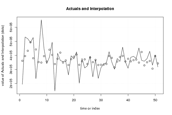
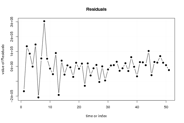
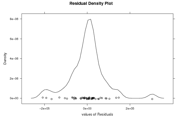
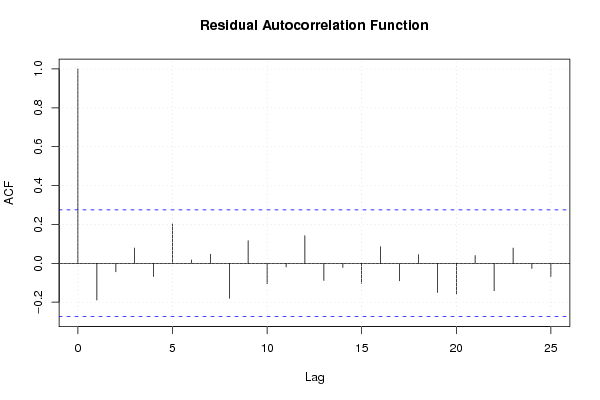
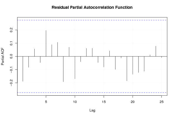
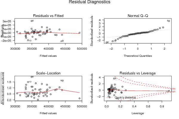
Charts produced by software:

http://www.freestatistics.org/blog/date/2010/Nov/30/t1291122381039j728zuhw8wg8/10n8b71291122137.png (open in new window) http://www.freestatistics.org/blog/date/2010/Nov/30/t1291122381039j728zuhw8wg8/10n8b71291122137.ps (open in new window) http://www.freestatistics.org/blog/date/2010/Nov/30/t1291122381039j728zuhw8wg8/1z7ed1291122137.png (open in new window) http://www.freestatistics.org/blog/date/2010/Nov/30/t1291122381039j728zuhw8wg8/1z7ed1291122137.ps (open in new window) http://www.freestatistics.org/blog/date/2010/Nov/30/t1291122381039j728zuhw8wg8/2rgvg1291122137.png (open in new window) http://www.freestatistics.org/blog/date/2010/Nov/30/t1291122381039j728zuhw8wg8/2rgvg1291122137.ps (open in new window) http://www.freestatistics.org/blog/date/2010/Nov/30/t1291122381039j728zuhw8wg8/3rgvg1291122137.png (open in new window) http://www.freestatistics.org/blog/date/2010/Nov/30/t1291122381039j728zuhw8wg8/3rgvg1291122137.ps (open in new window) http://www.freestatistics.org/blog/date/2010/Nov/30/t1291122381039j728zuhw8wg8/4rgvg1291122137.png (open in new window) http://www.freestatistics.org/blog/date/2010/Nov/30/t1291122381039j728zuhw8wg8/4rgvg1291122137.ps (open in new window) http://www.freestatistics.org/blog/date/2010/Nov/30/t1291122381039j728zuhw8wg8/5k8d11291122137.png (open in new window) http://www.freestatistics.org/blog/date/2010/Nov/30/t1291122381039j728zuhw8wg8/5k8d11291122137.ps (open in new window) http://www.freestatistics.org/blog/date/2010/Nov/30/t1291122381039j728zuhw8wg8/6k8d11291122137.png (open in new window) http://www.freestatistics.org/blog/date/2010/Nov/30/t1291122381039j728zuhw8wg8/6k8d11291122137.ps (open in new window) http://www.freestatistics.org/blog/date/2010/Nov/30/t1291122381039j728zuhw8wg8/7vzc41291122137.png (open in new window) http://www.freestatistics.org/blog/date/2010/Nov/30/t1291122381039j728zuhw8wg8/7vzc41291122137.ps (open in new window) http://www.freestatistics.org/blog/date/2010/Nov/30/t1291122381039j728zuhw8wg8/8vzc41291122137.png (open in new window) http://www.freestatistics.org/blog/date/2010/Nov/30/t1291122381039j728zuhw8wg8/8vzc41291122137.ps (open in new window) http://www.freestatistics.org/blog/date/2010/Nov/30/t1291122381039j728zuhw8wg8/9n8b71291122137.png (open in new window) http://www.freestatistics.org/blog/date/2010/Nov/30/t1291122381039j728zuhw8wg8/9n8b71291122137.ps (open in new window)

Parameters (Session):

par1 = 5 ; par2 = Do not include Seasonal Dummies ; par3 = No Linear Trend ;

Parameters (R input):

par1 = 5 ; par2 = Do not include Seasonal Dummies ; par3 = No Linear Trend ;

R code (references can be found in the software module):

library(lattice) library(lmtest) n25 <- 25 #minimum number of obs. for Goldfeld-Quandt test par1 <- as.numeric(par1) x <- t(y) k <- length(x[1,]) n <- length(x[,1]) x1 <- cbind(x[,par1], x[,1:k!=par1]) mycolnames <- c(colnames(x)[par1], colnames(x)[1:k!=par1]) colnames(x1) <- mycolnames #colnames(x)[par1] x <- x1 if (par3 == 'First Differences'){ x2 <- array(0, dim=c(n-1,k), dimnames=list(1:(n-1), paste('(1-B)',colnames(x),sep=''))) for (i in 1:n-1) { for (j in 1:k) { x2[i,j] <- x[i+1,j] - x[i,j] } } x <- x2 } if (par2 == 'Include Monthly Dummies'){ x2 <- array(0, dim=c(n,11), dimnames=list(1:n, paste('M', seq(1:11), sep =''))) for (i in 1:11){ x2[seq(i,n,12),i] <- 1 } x <- cbind(x, x2) } if (par2 == 'Include Quarterly Dummies'){ x2 <- array(0, dim=c(n,3), dimnames=list(1:n, paste('Q', seq(1:3), sep =''))) for (i in 1:3){ x2[seq(i,n,4),i] <- 1 } x <- cbind(x, x2) } k <- length(x[1,]) if (par3 == 'Linear Trend'){ x <- cbind(x, c(1:n)) colnames(x)[k+1] <- 't' } x k <- length(x[1,]) df <- as.data.frame(x) (mylm <- lm(df)) (mysum <- summary(mylm)) if (n > n25) { kp3 <- k + 3 nmkm3 <- n - k - 3 gqarr <- array(NA, dim=c(nmkm3-kp3+1,3)) numgqtests <- 0 numsignificant1 <- 0 numsignificant5 <- 0 numsignificant10 <- 0 for (mypoint in kp3:nmkm3) { j <- 0 numgqtests <- numgqtests + 1 for (myalt in c('greater', 'two.sided', 'less')) { j <- j + 1 gqarr[mypoint-kp3+1,j] <- gqtest(mylm, point=mypoint, alternative=myalt)$p.value } if (gqarr[mypoint-kp3+1,2] < 0.01) numsignificant1 <- numsignificant1 + 1 if (gqarr[mypoint-kp3+1,2] < 0.05) numsignificant5 <- numsignificant5 + 1 if (gqarr[mypoint-kp3+1,2] < 0.10) numsignificant10 <- numsignificant10 + 1 } gqarr } bitmap(file='test0.png') plot(x[,1], type='l', main='Actuals and Interpolation', ylab='value of Actuals and Interpolation (dots)', xlab='time or index') points(x[,1]-mysum$resid) grid() dev.off() bitmap(file='test1.png') plot(mysum$resid, type='b', pch=19, main='Residuals', ylab='value of Residuals', xlab='time or index') grid() dev.off() bitmap(file='test2.png') hist(mysum$resid, main='Residual Histogram', xlab='values of Residuals') grid() dev.off() bitmap(file='test3.png') densityplot(~mysum$resid,col='black',main='Residual Density Plot', xlab='values of Residuals') dev.off() bitmap(file='test4.png') qqnorm(mysum$resid, main='Residual Normal Q-Q Plot') qqline(mysum$resid) grid() dev.off() (myerror <- as.ts(mysum$resid)) bitmap(file='test5.png') dum <- cbind(lag(myerror,k=1),myerror) dum dum1 <- dum[2:length(myerror),] dum1 z <- as.data.frame(dum1) z plot(z,main=paste('Residual Lag plot, lowess, and regression line'), ylab='values of Residuals', xlab='lagged values of Residuals') lines(lowess(z)) abline(lm(z)) grid() dev.off() bitmap(file='test6.png') acf(mysum$resid, lag.max=length(mysum$resid)/2, main='Residual Autocorrelation Function') grid() dev.off() bitmap(file='test7.png') pacf(mysum$resid, lag.max=length(mysum$resid)/2, main='Residual Partial Autocorrelation Function') grid() dev.off() bitmap(file='test8.png') opar <- par(mfrow = c(2,2), oma = c(0, 0, 1.1, 0)) plot(mylm, las = 1, sub='Residual Diagnostics') par(opar) dev.off() if (n > n25) { bitmap(file='test9.png') plot(kp3:nmkm3,gqarr[,2], main='Goldfeld-Quandt test',ylab='2-sided p-value',xlab='breakpoint') grid() dev.off() } load(file='createtable') a<-table.start() a<-table.row.start(a) a<-table.element(a, 'Multiple Linear Regression - Estimated Regression Equation', 1, TRUE) a<-table.row.end(a) myeq <- colnames(x)[1] myeq <- paste(myeq, '[t] = ', sep='') for (i in 1:k){ if (mysum$coefficients[i,1] > 0) myeq <- paste(myeq, '+', '') myeq <- paste(myeq, mysum$coefficients[i,1], sep=' ') if (rownames(mysum$coefficients)[i] != '(Intercept)') { myeq <- paste(myeq, rownames(mysum$coefficients)[i], sep='') if (rownames(mysum$coefficients)[i] != 't') myeq <- paste(myeq, '[t]', sep='') } } myeq <- paste(myeq, ' + e[t]') a<-table.row.start(a) a<-table.element(a, myeq) a<-table.row.end(a) a<-table.end(a) table.save(a,file='mytable1.tab') a<-table.start() a<-table.row.start(a) a<-table.element(a,hyperlink('http://www.xycoon.com/ols1.htm','Multiple Linear Regression - Ordinary Least Squares',''), 6, TRUE) a<-table.row.end(a) a<-table.row.start(a) a<-table.element(a,'Variable',header=TRUE) a<-table.element(a,'Parameter',header=TRUE) a<-table.element(a,'S.D.',header=TRUE) a<-table.element(a,'T-STAT<br />H0: parameter = 0',header=TRUE) a<-table.element(a,'2-tail p-value',header=TRUE) a<-table.element(a,'1-tail p-value',header=TRUE) a<-table.row.end(a) for (i in 1:k){ a<-table.row.start(a) a<-table.element(a,rownames(mysum$coefficients)[i],header=TRUE) a<-table.element(a,mysum$coefficients[i,1]) a<-table.element(a, round(mysum$coefficients[i,2],6)) a<-table.element(a, round(mysum$coefficients[i,3],4)) a<-table.element(a, round(mysum$coefficients[i,4],6)) a<-table.element(a, round(mysum$coefficients[i,4]/2,6)) a<-table.row.end(a) } a<-table.end(a) table.save(a,file='mytable2.tab') a<-table.start() a<-table.row.start(a) a<-table.element(a, 'Multiple Linear Regression - Regression Statistics', 2, TRUE) a<-table.row.end(a) a<-table.row.start(a) a<-table.element(a, 'Multiple R',1,TRUE) a<-table.element(a, sqrt(mysum$r.squared)) a<-table.row.end(a) a<-table.row.start(a) a<-table.element(a, 'R-squared',1,TRUE) a<-table.element(a, mysum$r.squared) a<-table.row.end(a) a<-table.row.start(a) a<-table.element(a, 'Adjusted R-squared',1,TRUE) a<-table.element(a, mysum$adj.r.squared) a<-table.row.end(a) a<-table.row.start(a) a<-table.element(a, 'F-TEST (value)',1,TRUE) a<-table.element(a, mysum$fstatistic[1]) a<-table.row.end(a) a<-table.row.start(a) a<-table.element(a, 'F-TEST (DF numerator)',1,TRUE) a<-table.element(a, mysum$fstatistic[2]) a<-table.row.end(a) a<-table.row.start(a) a<-table.element(a, 'F-TEST (DF denominator)',1,TRUE) a<-table.element(a, mysum$fstatistic[3]) a<-table.row.end(a) a<-table.row.start(a) a<-table.element(a, 'p-value',1,TRUE) a<-table.element(a, 1-pf(mysum$fstatistic[1],mysum$fstatistic[2],mysum$fstatistic[3])) a<-table.row.end(a) a<-table.row.start(a) a<-table.element(a, 'Multiple Linear Regression - Residual Statistics', 2, TRUE) a<-table.row.end(a) a<-table.row.start(a) a<-table.element(a, 'Residual Standard Deviation',1,TRUE) a<-table.element(a, mysum$sigma) a<-table.row.end(a) a<-table.row.start(a) a<-table.element(a, 'Sum Squared Residuals',1,TRUE) a<-table.element(a, sum(myerror*myerror)) a<-table.row.end(a) a<-table.end(a) table.save(a,file='mytable3.tab') a<-table.start() a<-table.row.start(a) a<-table.element(a, 'Multiple Linear Regression - Actuals, Interpolation, and Residuals', 4, TRUE) a<-table.row.end(a) a<-table.row.start(a) a<-table.element(a, 'Time or Index', 1, TRUE) a<-table.element(a, 'Actuals', 1, TRUE) a<-table.element(a, 'Interpolation<br />Forecast', 1, TRUE) a<-table.element(a, 'Residuals<br />Prediction Error', 1, TRUE) a<-table.row.end(a) for (i in 1:n) { a<-table.row.start(a) a<-table.element(a,i, 1, TRUE) a<-table.element(a,x[i]) a<-table.element(a,x[i]-mysum$resid[i]) a<-table.element(a,mysum$resid[i]) a<-table.row.end(a) } a<-table.end(a) table.save(a,file='mytable4.tab') if (n > n25) { a<-table.start() a<-table.row.start(a) a<-table.element(a,'Goldfeld-Quandt test for Heteroskedasticity',4,TRUE) a<-table.row.end(a) a<-table.row.start(a) a<-table.element(a,'p-values',header=TRUE) a<-table.element(a,'Alternative Hypothesis',3,header=TRUE) a<-table.row.end(a) a<-table.row.start(a) a<-table.element(a,'breakpoint index',header=TRUE) a<-table.element(a,'greater',header=TRUE) a<-table.element(a,'2-sided',header=TRUE) a<-table.element(a,'less',header=TRUE) a<-table.row.end(a) for (mypoint in kp3:nmkm3) { a<-table.row.start(a) a<-table.element(a,mypoint,header=TRUE) a<-table.element(a,gqarr[mypoint-kp3+1,1]) a<-table.element(a,gqarr[mypoint-kp3+1,2]) a<-table.element(a,gqarr[mypoint-kp3+1,3]) a<-table.row.end(a) } a<-table.end(a) table.save(a,file='mytable5.tab') a<-table.start() a<-table.row.start(a) a<-table.element(a,'Meta Analysis of Goldfeld-Quandt test for Heteroskedasticity',4,TRUE) a<-table.row.end(a) a<-table.row.start(a) a<-table.element(a,'Description',header=TRUE) a<-table.element(a,'# significant tests',header=TRUE) a<-table.element(a,'% significant tests',header=TRUE) a<-table.element(a,'OK/NOK',header=TRUE) a<-table.row.end(a) a<-table.row.start(a) a<-table.element(a,'1% type I error level',header=TRUE) a<-table.element(a,numsignificant1) a<-table.element(a,numsignificant1/numgqtests) if (numsignificant1/numgqtests < 0.01) dum <- 'OK' else dum <- 'NOK' a<-table.element(a,dum) a<-table.row.end(a) a<-table.row.start(a) a<-table.element(a,'5% type I error level',header=TRUE) a<-table.element(a,numsignificant5) a<-table.element(a,numsignificant5/numgqtests) if (numsignificant5/numgqtests < 0.05) dum <- 'OK' else dum <- 'NOK' a<-table.element(a,dum) a<-table.row.end(a) a<-table.row.start(a) a<-table.element(a,'10% type I error level',header=TRUE) a<-table.element(a,numsignificant10) a<-table.element(a,numsignificant10/numgqtests) if (numsignificant10/numgqtests < 0.1) dum <- 'OK' else dum <- 'NOK' a<-table.element(a,dum) a<-table.row.end(a) a<-table.end(a) table.save(a,file='mytable6.tab') }

Copyright

This work is licensed under a Creative Commons Attribution-Noncommercial-Share Alike 3.0 License.

Software written by Ed van Stee & Patrick Wessa

Disclaimer

Information provided on this web site is provided "AS IS" without warranty of any kind, either express or implied, including, without limitation, warranties of merchantability, fitness for a particular purpose, and noninfringement. We use reasonable efforts to include accurate and timely information and periodically update the information, and software without notice. However, we make no warranties or representations as to the accuracy or completeness of such information (or software), and we assume no liability or responsibility for errors or omissions in the content of this web site, or any software bugs in online applications. Your use of this web site is AT YOUR OWN RISK. Under no circumstances and under no legal theory shall we be liable to you or any other person for any direct, indirect, special, incidental, exemplary, or consequential damages arising from your access to, or use of, this web site.

Privacy Policy

We may request personal information to be submitted to our servers in order to be able to:

• personalize online software applications according to your needs
• enforce strict security rules with respect to the data that you upload (e.g. statistical data)
• manage user sessions of online applications
• alert you about important changes or upgrades in resources or applications

We NEVER allow other companies to directly offer registered users information about their products and services. Banner references and hyperlinks of third parties NEVER contain any personal data of the visitor.

We do NOT sell, nor transmit by any means, personal information, nor statistical data series uploaded by you to third parties.

We carefully protect your data from loss, misuse, alteration, and destruction. However, at any time, and under any circumstance you are solely responsible for managing your passwords, and keeping them secret.

We store a unique ANONYMOUS USER ID in the form of a small 'Cookie' on your computer. This allows us to track your progress when using this website which is necessary to create state-dependent features. The cookie is used for NO OTHER PURPOSE. At any time you may opt to disallow cookies from this website - this will not affect other features of this website.

We examine cookies that are used by third-parties (banner and online ads) very closely: abuse from third-parties automatically results in termination of the advertising contract without refund. We have very good reason to believe that the cookies that are produced by third parties (banner ads) do NOT cause any privacy or security risk.

FreeStatistics.org is safe. There is no need to download any software to use the applications and services contained in this website. Hence, your system's security is not compromised by their use, and your personal data - other than data you submit in the account application form, and the user-agent information that is transmitted by your browser - is never transmitted to our servers.

As a general rule, we do not log on-line behavior of individuals (other than normal logging of webserver 'hits'). However, in cases of abuse, hacking, unauthorized access, Denial of Service attacks, illegal copying, hotlinking, non-compliance with international webstandards (such as robots.txt), or any other harmful behavior, our system engineers are empowered to log, track, identify, publish, and ban misbehaving individuals - even if this leads to ban entire blocks of IP addresses, or disclosing user's identity.

FreeStatistics.org is powered by