Free Statistics
of Irreproducible Research!
Description of Statistical Computation | |||||||||||||||||||||
|---|---|---|---|---|---|---|---|---|---|---|---|---|---|---|---|---|---|---|---|---|---|
| Author's title | |||||||||||||||||||||
| Author | *Unverified author* | ||||||||||||||||||||
| R Software Module | rwasp_meanplot.wasp | ||||||||||||||||||||
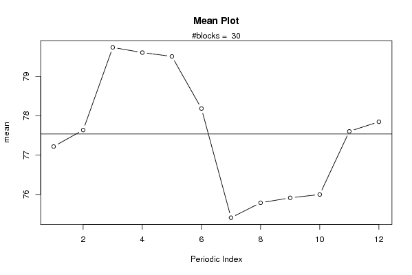
| Title produced by software | Mean Plot | ||||||||||||||||||||
| Date of computation | Mon, 07 Jan 2008 06:38:24 -0700 | ||||||||||||||||||||
| Cite this page as follows | Statistical Computations at FreeStatistics.org, Office for Research Development and Education, URL https://freestatistics.org/blog/index.php?v=date/2008/Jan/07/t119971350673encrjvyxgcqw7.htm/, Retrieved Fri, 19 Apr 2024 00:43:24 +0000 | ||||||||||||||||||||
| Statistical Computations at FreeStatistics.org, Office for Research Development and Education, URL https://freestatistics.org/blog/index.php?pk=7917, Retrieved Fri, 19 Apr 2024 00:43:24 +0000 | |||||||||||||||||||||
| QR Codes: | |||||||||||||||||||||
|
| |||||||||||||||||||||
| Original text written by user: | |||||||||||||||||||||
| IsPrivate? | No (this computation is public) | ||||||||||||||||||||
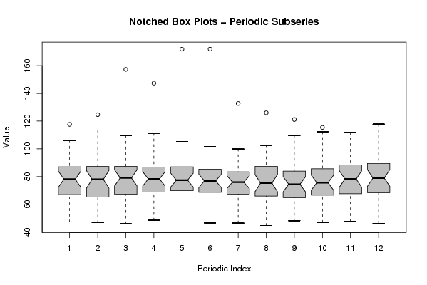
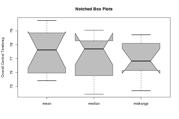
| User-defined keywords | mean, median, midrange, mean plot, seasonality, trend | ||||||||||||||||||||
| Estimated Impact | 36 | ||||||||||||||||||||
Tree of Dependent Computations | |||||||||||||||||||||
| Family? (F = Feedback message, R = changed R code, M = changed R Module, P = changed Parameters, D = changed Data) | |||||||||||||||||||||
| - [Bivariate Data Series] [Bivariate dataset] [2008-01-05 23:51:08] [74be16979710d4c4e7c6647856088456] F RMPD [Mean Plot] [Colombia Coffee] [2008-01-07 13:38:24] [d41d8cd98f00b204e9800998ecf8427e] [Current] - RMPD [Harrell-Davis Quantiles] [steve] [2008-04-15 18:01:58] [74be16979710d4c4e7c6647856088456] - PD [Mean Plot] [Notched boxplot -...] [2008-12-07 09:49:05] [c45c87b96bbf32ffc2144fc37d767b2e] - RMPD [Central Tendency] [central tendency] [2008-12-14 12:46:40] [c45c87b96bbf32ffc2144fc37d767b2e] - D [Central Tendency] [trimmed mean] [2008-12-16 21:19:25] [c45c87b96bbf32ffc2144fc37d767b2e] - D [Mean Plot] [Notched boxplot -...] [2008-12-14 12:56:52] [74be16979710d4c4e7c6647856088456] - D [Mean Plot] [Notched boxplot -...] [2008-12-16 21:22:54] [c45c87b96bbf32ffc2144fc37d767b2e] - M D [Mean Plot] [] [2009-12-30 10:19:42] [d2d412c7f4d35ffbf5ee5ee89db327d4] - D [Mean Plot] [] [2009-12-30 14:08:44] [d2d412c7f4d35ffbf5ee5ee89db327d4] - PD [Mean Plot] [Mean Plot - Xt - ...] [2008-12-22 10:24:52] [33f4701c7363e8b81858dafbf0350eed] - D [Mean Plot] [Mean Plot - Trans...] [2008-12-22 13:53:01] [33f4701c7363e8b81858dafbf0350eed] - D [Mean Plot] [Mean Plot - Trans...] [2008-12-22 20:19:36] [b187fac1a1b0cb3920f54366df47fea3] - D [Mean Plot] [mean plot - trans...] [2008-12-22 20:40:06] [b641c14ac36cb6fee377f3b099dcac19] - D [Mean Plot] [Mean Plot - Xt - ...] [2008-12-22 20:11:47] [b187fac1a1b0cb3920f54366df47fea3] - D [Mean Plot] [mean plot - Xt - ...] [2008-12-22 20:23:09] [b641c14ac36cb6fee377f3b099dcac19] - MPD [Mean Plot] [Workshop 6 assign...] [2010-11-05 08:31:09] [56d90b683fcd93137645f9226b43c62b] - MPD [Mean Plot] [W6 Assignments Tu...] [2010-11-05 08:36:37] [56d90b683fcd93137645f9226b43c62b] - MPD [Mean Plot] [WS6: Toturial ass...] [2010-11-05 10:06:39] [1fd136673b2a4fecb5c545b9b4a05d64] - P [Mean Plot] [ws6.2 tutorial (s...] [2010-11-15 08:09:29] [e4076051fbfb461c886b1e223cd7862f] - P [Mean Plot] [ws6.2 tutorial (f...] [2010-11-15 08:14:30] [e4076051fbfb461c886b1e223cd7862f] - RM [Mean Plot] [seasonality] [2011-11-15 14:45:19] [d31984dff2665bea309b726bae3d5241] - RM [Mean Plot] [forecasts acceptable] [2011-11-15 14:48:59] [d31984dff2665bea309b726bae3d5241] - RM [Mean Plot] [] [2011-11-15 21:53:28] [74be16979710d4c4e7c6647856088456] - RM [Mean Plot] [] [2011-11-15 21:59:12] [74be16979710d4c4e7c6647856088456] - MPD [Mean Plot] [Retailprijs - Sei...] [2010-11-05 10:26:46] [aeb27d5c05332f2e597ad139ee63fbe4] - D [Mean Plot] [Mean Plot - Niet ...] [2010-11-12 11:43:04] [aeb27d5c05332f2e597ad139ee63fbe4] - D [Mean Plot] [Mean Plot – Nie...] [2010-12-17 13:44:39] [aeb27d5c05332f2e597ad139ee63fbe4] - D [Mean Plot] [Mean Plot - VDAB ...] [2010-11-12 11:44:22] [aeb27d5c05332f2e597ad139ee63fbe4] - RMPD [Mean Plot] [WS6 - Simple Line...] [2010-11-05 13:17:47] [1f5baf2b24e732d76900bb8178fc04e7] - RMPD [Mean Plot] [Yt Seasonality] [2010-11-05 16:54:03] [97ad38b1c3b35a5feca8b85f7bc7b3ff] - PD [Mean Plot] [Vraag 2: seasonality] [2010-11-11 09:55:50] [39c51da0be01189e8a44eb69e891b7a1] - R PD [Mean Plot] [] [2010-11-16 17:11:22] [8ef75e99f9f5061c72c54640f2f1c3e7] F D [Mean Plot] [ws6] [2010-11-17 09:01:38] [f9eaed74daea918f73b9f505c5b1f19e] F D [Mean Plot] [ws6] [2010-11-17 09:03:07] [f9eaed74daea918f73b9f505c5b1f19e] - RM [Mean Plot] [WS 6 - 9] [2011-11-15 14:49:53] [74be16979710d4c4e7c6647856088456] - R D [Mean Plot] [C6 A2.2] [2011-11-15 15:38:45] [d1ce18d003fa52f731d1c3ce8b58d5f9] - R PD [Mean Plot] [] [2011-11-15 20:18:15] [ec2187f7727da5d5d939740b21b8b68a] - R PD [Mean Plot] [] [2011-11-15 20:19:06] [ec2187f7727da5d5d939740b21b8b68a] - MPD [Mean Plot] [WS6 - Assignment ...] [2010-11-06 11:08:15] [8ef49741e164ec6343c90c7935194465] - P [Mean Plot] [WS6 assignment 2 ...] [2010-11-16 20:16:02] [8214fe6d084e5ad7598b249a26cc9f06] - P [Mean Plot] [WS6 assignment 2 ...] [2010-11-16 20:17:31] [8214fe6d084e5ad7598b249a26cc9f06] - P [Mean Plot] [] [2010-11-17 09:46:18] [afdb2fc47981b6a655b732edc8065db9] - MPD [Mean Plot] [] [2010-11-06 13:07:35] [39e83c7b0ac936e906a817a1bb402750] - RMPD [Mean Plot] [Mean Plot Car sales] [2010-11-06 16:22:27] [97ad38b1c3b35a5feca8b85f7bc7b3ff] - D [Mean Plot] [Mean Plot Gasolin...] [2010-11-06 16:47:42] [97ad38b1c3b35a5feca8b85f7bc7b3ff] - R D [Mean Plot] [] [2011-11-15 17:01:45] [06c08141d7d783218a8164fd2ea166f2] - R P [Mean Plot] [] [2011-11-15 21:34:25] [ec2187f7727da5d5d939740b21b8b68a] - R D [Mean Plot] [] [2011-11-15 15:57:49] [06c08141d7d783218a8164fd2ea166f2] - D [Mean Plot] [] [2011-12-20 18:10:55] [06c08141d7d783218a8164fd2ea166f2] [Truncated] | |||||||||||||||||||||
| Feedback Forum | |||||||||||||||||||||
Post a new message | |||||||||||||||||||||
Dataset | |||||||||||||||||||||
| Dataseries X: | |||||||||||||||||||||
87.28 87.28 87.09 86.92 87.59 90.72 90.69 90.3 89.55 88.94 88.41 87.82 87.07 86.82 86.4 86.02 85.66 85.32 85 84.67 83.94 82.83 81.95 81.19 80.48 78.86 69.47 68.77 70.06 73.95 75.8 77.79 81.57 83.07 84.34 85.1 85.25 84.26 83.63 86.44 85.3 84.1 83.36 82.48 81.58 80.47 79.34 82.13 81.69 80.7 79.88 79.16 78.38 77.42 76.47 75.46 74.48 78.27 80.7 79.91 78.75 77.78 81.14 81.08 80.03 78.91 78.01 76.9 75.97 81.93 80.27 78.67 77.42 76.16 74.7 76.39 76.04 74.65 73.29 71.79 74.39 74.91 74.54 73.08 72.75 71.32 70.38 70.35 70.01 69.36 67.77 69.26 69.8 68.38 67.62 68.39 66.95 65.21 66.64 63.45 60.66 62.34 60.32 58.64 60.46 58.59 61.87 61.85 67.44 77.06 91.74 93.15 94.15 93.11 91.51 89.96 88.16 86.98 88.03 86.24 84.65 83.23 81.7 80.25 78.8 77.51 76.2 75.04 74 75.49 77.14 76.15 76.27 78.19 76.49 77.31 76.65 74.99 73.51 72.07 70.59 71.96 76.29 74.86 74.93 71.9 71.01 77.47 75.78 76.6 76.07 74.57 73.02 72.65 73.16 71.53 69.78 67.98 69.96 72.16 70.47 68.86 67.37 65.87 72.16 71.34 69.93 68.44 67.16 66.01 67.25 70.91 69.75 68.59 67.48 66.31 64.81 66.58 65.97 64.7 64.7 60.94 59.08 58.42 57.77 57.11 53.31 49.96 49.4 48.84 48.3 47.74 47.24 46.76 46.29 48.9 49.23 48.53 48.03 54.34 53.79 53.24 52.96 52.17 51.7 58.55 78.2 77.03 76.19 77.15 75.87 95.47 109.67 112.28 112.01 107.93 105.96 105.06 102.98 102.2 105.23 101.85 99.89 96.23 94.76 91.51 91.63 91.54 85.23 87.83 87.38 84.44 85.19 84.03 86.73 102.52 104.45 106.98 107.02 99.26 94.45 113.44 157.33 147.38 171.89 171.95 132.71 126.02 121.18 115.45 110.48 117.85 117.63 124.65 109.59 111.27 99.78 98.21 99.2 97.97 89.55 87.91 93.34 94.42 93.2 90.29 91.46 89.98 88.35 88.41 82.44 79.89 75.69 75.66 84.5 96.73 87.48 82.39 83.48 79.31 78.16 72.77 72.45 68.46 67.62 68.76 70.07 68.55 65.3 58.96 59.17 62.37 66.28 55.62 55.23 55.85 56.75 50.89 53.88 52.95 55.08 53.61 58.78 61.85 55.91 53.32 46.41 44.57 50 50 53.36 46.23 50.45 49.07 45.85 48.45 49.96 46.53 50.51 47.58 48.05 46.84 47.67 49.16 55.54 55.82 58.22 56.19 57.77 63.19 54.76 55.74 62.54 61.39 69.6 79.23 80 93.68 107.63 100.18 97.3 90.45 80.64 80.58 75.82 85.59 89.35 89.42 104.73 95.32 89.27 90.44 86.97 79.98 81.22 87.35 83.64 82.22 94.4 102.18 | |||||||||||||||||||||
Tables (Output of Computation) | |||||||||||||||||||||
| |||||||||||||||||||||
Figures (Output of Computation) | |||||||||||||||||||||
Input Parameters & R Code | |||||||||||||||||||||
| Parameters (Session): | |||||||||||||||||||||
| Parameters (R input): | |||||||||||||||||||||
| par1 = 12 ; | |||||||||||||||||||||
| R code (references can be found in the software module): | |||||||||||||||||||||
par1 <- as.numeric(par1) | |||||||||||||||||||||