| Multiple Linear Regression - Estimated Regression Equation |
| WINS[t] = -117.303237364796 + 847.806070695539OBP[t] -20.6264676476635ERA[t] -1.82894945319784M1[t] + 1.02461553276331M2[t] -1.47301486299800M3[t] + 5.68242881635786M4[t] + 2.21754466006933M5[t] + 1.30120128882525M6[t] -0.418959261383213M7[t] + 0.532020490334148M8[t] + 4.71778875876457M9[t] + 0.771801556313103M10[t] + 1.15700769424563M11[t] + e[t] |
| Multiple Linear Regression - Ordinary Least Squares | |||||
| Variable | Parameter | S.D. | T-STAT H0: parameter = 0 | 2-tail p-value | 1-tail p-value |
| (Intercept) | -117.303237364796 | 44.898079 | -2.6127 | 0.014501 | 0.007251 |
| OBP | 847.806070695539 | 159.615356 | 5.3116 | 1.3e-05 | 7e-06 |
| ERA | -20.6264676476635 | 4.459327 | -4.6255 | 8.3e-05 | 4.2e-05 |
| M1 | -1.82894945319784 | 7.451844 | -0.2454 | 0.807975 | 0.403988 |
| M2 | 1.02461553276331 | 7.416914 | 0.1381 | 0.89115 | 0.445575 |
| M3 | -1.47301486299800 | 7.515129 | -0.196 | 0.846073 | 0.423036 |
| M4 | 5.68242881635786 | 7.489977 | 0.7587 | 0.454622 | 0.227311 |
| M5 | 2.21754466006933 | 7.671775 | 0.2891 | 0.774749 | 0.387375 |
| M6 | 1.30120128882525 | 8.464763 | 0.1537 | 0.878974 | 0.439487 |
| M7 | -0.418959261383213 | 8.771789 | -0.0478 | 0.962257 | 0.481129 |
| M8 | 0.532020490334148 | 8.820851 | 0.0603 | 0.95235 | 0.476175 |
| M9 | 4.71778875876457 | 7.909659 | 0.5965 | 0.555837 | 0.277918 |
| M10 | 0.771801556313103 | 7.962074 | 0.0969 | 0.923494 | 0.461747 |
| M11 | 1.15700769424563 | 7.895271 | 0.1465 | 0.88458 | 0.44229 |
| Multiple Linear Regression - Regression Statistics | |
| Multiple R | 0.82960034298999 |
| R-squared | 0.688236729089108 |
| Adjusted R-squared | 0.53812848753942 |
| F-TEST (value) | 4.5849363231751 |
| F-TEST (DF numerator) | 13 |
| F-TEST (DF denominator) | 27 |
| p-value | 0.000411719452773518 |
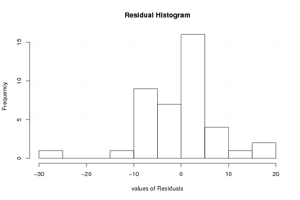
| Multiple Linear Regression - Residual Statistics | |
| Residual Standard Deviation | 9.65203279600039 |
| Sum Squared Residuals | 2515.36690156681 |
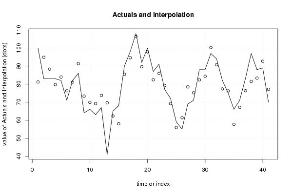
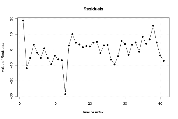
| Multiple Linear Regression - Actuals, Interpolation, and Residuals | |||
| Time or Index | Actuals | Interpolation Forecast | Residuals Prediction Error |
| 1 | 100 | 81.1667507604141 | 18.8332492395859 |
| 2 | 83 | 94.8794863251428 | -11.8794863251428 |
| 3 | 83 | 88.3051339161781 | -5.30513391617807 |
| 4 | 83 | 79.7177584823183 | 3.28224151768168 |
| 5 | 82 | 83.8831289622896 | -1.88312896228963 |
| 6 | 71 | 76.2753264846372 | -5.27532648463724 |
| 7 | 82 | 81.1086024587274 | 0.891397541272554 |
| 8 | 86 | 91.3414926518934 | -5.34149265189338 |
| 9 | 64 | 73.3204563485899 | -9.32045634858988 |
| 10 | 66 | 69.8552405934587 | -3.85524059345869 |
| 11 | 63 | 69.16362861943 | -6.16362861943003 |
| 12 | 67 | 73.7349987435766 | -6.73499874357655 |
| 13 | 41 | 69.6159288777224 | -28.6159288777224 |
| 14 | 65 | 62.2715352571724 | 2.7284647428276 |
| 15 | 68 | 57.964555896075 | 10.035444103925 |
| 16 | 90 | 85.4218505425458 | 4.57814945745418 |
| 17 | 98 | 94.607353745699 | 3.39264625430099 |
| 18 | 108 | 106.408101434888 | 1.59189856511197 |
| 19 | 92 | 89.6306195018852 | 2.36938049811477 |
| 20 | 100 | 97.894929176192 | 2.10507082380793 |
| 21 | 87 | 82.3733547487728 | 4.62664525122720 |
| 22 | 91 | 85.9195996004716 | 5.08040039952843 |
| 23 | 77 | 79.1780699142535 | -2.17806991425350 |
| 24 | 72 | 69.1759668896772 | 2.82403311032279 |
| 25 | 59 | 55.9114707711085 | 3.08852922889154 |
| 26 | 55 | 61.3539486987342 | -6.35394869873424 |
| 27 | 69 | 78.425638416713 | -9.42563841671297 |
| 28 | 71 | 75.176858813081 | -4.17685881308109 |
| 29 | 88 | 82.367957345835 | 5.63204265416507 |
| 30 | 88 | 84.3165720804747 | 3.68342791952526 |
| 31 | 97 | 100.260778039387 | -3.26077803938732 |
| 32 | 94 | 90.7635781719146 | 3.23642182808545 |
| 33 | 82 | 77.3061889026373 | 4.69381109736269 |
| 34 | 75 | 76.2251598060697 | -1.22515980606974 |
| 35 | 66 | 57.6583014663165 | 8.34169853368352 |
| 36 | 71 | 67.0890343667462 | 3.91096563325376 |
| 37 | 83 | 76.305849590755 | 6.69415040924496 |
| 38 | 97 | 81.4950297189506 | 15.5049702810494 |
| 39 | 88 | 83.304671771034 | 4.69532822896605 |
| 40 | 89 | 92.6835321620548 | -3.68353216205478 |
| 41 | 70 | 77.1415599461764 | -7.14155994617644 |
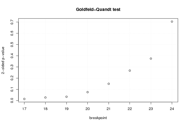
| Goldfeld-Quandt test for Heteroskedasticity | |||
| p-values | Alternative Hypothesis | ||
| breakpoint index | greater | 2-sided | less |
| 17 | 0.992622118255582 | 0.0147557634888352 | 0.0073778817444176 |
| 18 | 0.986209870430301 | 0.0275802591393977 | 0.0137901295696988 |
| 19 | 0.98264514146231 | 0.0347097170753798 | 0.0173548585376899 |
| 20 | 0.962285477583543 | 0.0754290448329142 | 0.0377145224164571 |
| 21 | 0.925040564786353 | 0.149918870427294 | 0.0749594352136468 |
| 22 | 0.866151329003894 | 0.267697341992212 | 0.133848670996106 |
| 23 | 0.812804825725631 | 0.374390348548738 | 0.187195174274369 |
| 24 | 0.647658723855137 | 0.704682552289727 | 0.352341276144863 |
| Meta Analysis of Goldfeld-Quandt test for Heteroskedasticity | |||
| Description | # significant tests | % significant tests | OK/NOK |
| 1% type I error level | 0 | 0 | OK |
| 5% type I error level | 3 | 0.375 | NOK |
| 10% type I error level | 4 | 0.5 | NOK |