Repository of Reproducible Computations

Free Statistics

of Irreproducible Research!

Author's title

Author

*The author of this computation has been verified*

R Software Module

rwasp_arimaforecasting.wasp

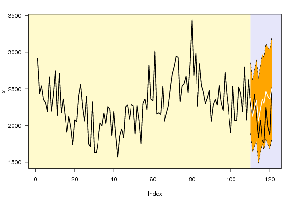
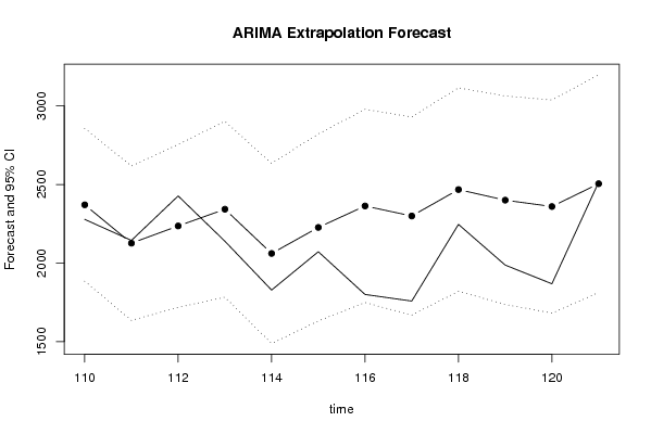
Title produced by software

ARIMA Forecasting

Date of computation

Thu, 10 Dec 2009 01:34:29 -0700

Cite this page as follows

Statistical Computations at FreeStatistics.org, Office for Research Development and Education, URL https://freestatistics.org/blog/index.php?v=date/2009/Dec/10/t1260434176ct288950nz2ldfx.htm/, Retrieved Wed, 24 Apr 2024 12:09:34 +0000

Statistical Computations at FreeStatistics.org, Office for Research Development and Education, URL https://freestatistics.org/blog/index.php?pk=65235, Retrieved Wed, 24 Apr 2024 12:09:34 +0000

QR Codes:

Paste this QR Code to cite your computation.

Original text written by user:

IsPrivate?

No (this computation is public)

User-defined keywords

Estimated Impact

167

Family? (F = Feedback message, R = changed R code, M = changed R Module, P = changed Parameters, D = changed Data)

-     [ARIMA Forecasting] [] [2009-12-07 09:54:52] [b98453cac15ba1066b407e146608df68]
- R PD  [ARIMA Forecasting] [ARIMA-Forecasting] [2009-12-09 16:48:03] [ee7c2e7343f5b1451e62c5c16ec521f1]
-   PD      [ARIMA Forecasting] [ARIMA forecasting] [2009-12-10 08:34:29] [865cd78857e928bd6e7d79509c6cdcc5] [Current]
-   P         [ARIMA Forecasting] [] [2009-12-10 10:17:58] [a542c511726eba04a1fc2f4bd37a90f8] 
-   PD        [ARIMA Forecasting] [Arima forecasting] [2009-12-11 20:47:14] [76ab39dc7a55316678260825bd5ad46c] 
-   PD          [ARIMA Forecasting] [ARIMA forecasting] [2009-12-11 22:18:44] [4b453aa14d54730625f8d3de5f1f6d82] 

Feedback Forum

Post a new message

Dataseries X:

Download CSV

Histogram

Boxplots

Summary of computational transaction
Raw Input	view raw input (R code)
Raw Output	view raw output of R engine
Computing time	2 seconds
R Server	'Gwilym Jenkins' @ 72.249.127.135

\begin{tabular}{lllllllll}
\hline
Summary of computational transaction \tabularnewline
Raw Input & view raw input (R code)  \tabularnewline
Raw Output & view raw output of R engine  \tabularnewline
Computing time & 2 seconds \tabularnewline
R Server & 'Gwilym Jenkins' @ 72.249.127.135 \tabularnewline
\hline
\end{tabular}
%Source: https://freestatistics.org/blog/index.php?pk=65235&T=0

[TABLE]
[ROW][C]Summary of computational transaction[/C][/ROW]
[ROW][C]Raw Input[/C][C]view raw input (R code) [/C][/ROW]
[ROW][C]Raw Output[/C][C]view raw output of R engine [/C][/ROW]
[ROW][C]Computing time[/C][C]2 seconds[/C][/ROW]
[ROW][C]R Server[/C][C]'Gwilym Jenkins' @ 72.249.127.135[/C][/ROW]
[/TABLE]
Source: https://freestatistics.org/blog/index.php?pk=65235&T=0

Globally Unique Identifier (entire table): ba.freestatistics.org/blog/index.php?pk=65235&T=0

As an alternative you can also use a QR Code:

The GUIDs for individual cells are displayed in the table below:

Summary of computational transaction
Raw Input	view raw input (R code)
Raw Output	view raw output of R engine
Computing time	2 seconds
R Server	'Gwilym Jenkins' @ 72.249.127.135

Univariate ARIMA Extrapolation Forecast
time	Y[t]	F[t]	95% LB	95% UB	p-value(H0: Y[t] = F[t])	P(F[t]>Y[t-1])	P(F[t]>Y[t-s])	P(F[t]>Y[109])
97	2725	-	-	-	-	-	-	-
98	2408	-	-	-	-	-	-	-
99	2139	-	-	-	-	-	-	-
100	1898	-	-	-	-	-	-	-
101	2537	-	-	-	-	-	-	-
102	2069	-	-	-	-	-	-	-
103	2063	-	-	-	-	-	-	-
104	2524	-	-	-	-	-	-	-
105	2437	-	-	-	-	-	-	-
106	2189	-	-	-	-	-	-	-
107	2793	-	-	-	-	-	-	-
108	2074	-	-	-	-	-	-	-
109	2622	-	-	-	-	-	-	-
110	2278	2370.6852	1884.4469	2856.9234	0.3543	0.1555	0.4402	0.1555
111	2144	2126.3999	1635.2867	2617.5131	0.472	0.2726	0.4799	0.024
112	2427	2235.914	1717.5708	2754.2572	0.235	0.6359	0.8993	0.0722
113	2139	2342.5471	1782.7686	2902.3256	0.238	0.3837	0.248	0.1639
114	1828	2061.0709	1487.5664	2634.5754	0.2129	0.395	0.4892	0.0276
115	2072	2226.6978	1631.5596	2821.8361	0.3052	0.9054	0.7051	0.0965
116	1800	2363.2324	1748.3799	2978.0849	0.0363	0.8234	0.3042	0.2047
117	1758	2299.5048	1669.0944	2929.9152	0.0461	0.9398	0.3345	0.158
118	2246	2467.7044	1820.2081	3115.2007	0.2511	0.9842	0.8006	0.3202
119	1987	2400.1313	1736.9244	3063.3381	0.1111	0.6756	0.1228	0.256
120	1868	2359.6613	1681.6421	3037.6805	0.0776	0.8593	0.7955	0.2241
121	2514	2504.8962	1811.8224	3197.9699	0.4897	0.9642	0.3703	0.3703

\begin{tabular}{lllllllll}
\hline
Univariate ARIMA Extrapolation Forecast \tabularnewline
time & Y[t] & F[t] & 95% LB & 95% UB & p-value(H0: Y[t] = F[t]) & P(F[t]>Y[t-1]) & P(F[t]>Y[t-s]) & P(F[t]>Y[109]) \tabularnewline
97 & 2725 & - & - & - & - & - & - & - \tabularnewline
98 & 2408 & - & - & - & - & - & - & - \tabularnewline
99 & 2139 & - & - & - & - & - & - & - \tabularnewline
100 & 1898 & - & - & - & - & - & - & - \tabularnewline
101 & 2537 & - & - & - & - & - & - & - \tabularnewline
102 & 2069 & - & - & - & - & - & - & - \tabularnewline
103 & 2063 & - & - & - & - & - & - & - \tabularnewline
104 & 2524 & - & - & - & - & - & - & - \tabularnewline
105 & 2437 & - & - & - & - & - & - & - \tabularnewline
106 & 2189 & - & - & - & - & - & - & - \tabularnewline
107 & 2793 & - & - & - & - & - & - & - \tabularnewline
108 & 2074 & - & - & - & - & - & - & - \tabularnewline
109 & 2622 & - & - & - & - & - & - & - \tabularnewline
110 & 2278 & 2370.6852 & 1884.4469 & 2856.9234 & 0.3543 & 0.1555 & 0.4402 & 0.1555 \tabularnewline
111 & 2144 & 2126.3999 & 1635.2867 & 2617.5131 & 0.472 & 0.2726 & 0.4799 & 0.024 \tabularnewline
112 & 2427 & 2235.914 & 1717.5708 & 2754.2572 & 0.235 & 0.6359 & 0.8993 & 0.0722 \tabularnewline
113 & 2139 & 2342.5471 & 1782.7686 & 2902.3256 & 0.238 & 0.3837 & 0.248 & 0.1639 \tabularnewline
114 & 1828 & 2061.0709 & 1487.5664 & 2634.5754 & 0.2129 & 0.395 & 0.4892 & 0.0276 \tabularnewline
115 & 2072 & 2226.6978 & 1631.5596 & 2821.8361 & 0.3052 & 0.9054 & 0.7051 & 0.0965 \tabularnewline
116 & 1800 & 2363.2324 & 1748.3799 & 2978.0849 & 0.0363 & 0.8234 & 0.3042 & 0.2047 \tabularnewline
117 & 1758 & 2299.5048 & 1669.0944 & 2929.9152 & 0.0461 & 0.9398 & 0.3345 & 0.158 \tabularnewline
118 & 2246 & 2467.7044 & 1820.2081 & 3115.2007 & 0.2511 & 0.9842 & 0.8006 & 0.3202 \tabularnewline
119 & 1987 & 2400.1313 & 1736.9244 & 3063.3381 & 0.1111 & 0.6756 & 0.1228 & 0.256 \tabularnewline
120 & 1868 & 2359.6613 & 1681.6421 & 3037.6805 & 0.0776 & 0.8593 & 0.7955 & 0.2241 \tabularnewline
121 & 2514 & 2504.8962 & 1811.8224 & 3197.9699 & 0.4897 & 0.9642 & 0.3703 & 0.3703 \tabularnewline
\hline
\end{tabular}
%Source: https://freestatistics.org/blog/index.php?pk=65235&T=1

[TABLE]
[ROW][C]Univariate ARIMA Extrapolation Forecast[/C][/ROW]
[ROW][C]time[/C][C]Y[t][/C][C]F[t][/C][C]95% LB[/C][C]95% UB[/C][C]p-value(H0: Y[t] = F[t])[/C][C]P(F[t]>Y[t-1])[/C][C]P(F[t]>Y[t-s])[/C][C]P(F[t]>Y[109])[/C][/ROW]
[ROW][C]97[/C][C]2725[/C][C]-[/C][C]-[/C][C]-[/C][C]-[/C][C]-[/C][C]-[/C][C]-[/C][/ROW]
[ROW][C]98[/C][C]2408[/C][C]-[/C][C]-[/C][C]-[/C][C]-[/C][C]-[/C][C]-[/C][C]-[/C][/ROW]
[ROW][C]99[/C][C]2139[/C][C]-[/C][C]-[/C][C]-[/C][C]-[/C][C]-[/C][C]-[/C][C]-[/C][/ROW]
[ROW][C]100[/C][C]1898[/C][C]-[/C][C]-[/C][C]-[/C][C]-[/C][C]-[/C][C]-[/C][C]-[/C][/ROW]
[ROW][C]101[/C][C]2537[/C][C]-[/C][C]-[/C][C]-[/C][C]-[/C][C]-[/C][C]-[/C][C]-[/C][/ROW]
[ROW][C]102[/C][C]2069[/C][C]-[/C][C]-[/C][C]-[/C][C]-[/C][C]-[/C][C]-[/C][C]-[/C][/ROW]
[ROW][C]103[/C][C]2063[/C][C]-[/C][C]-[/C][C]-[/C][C]-[/C][C]-[/C][C]-[/C][C]-[/C][/ROW]
[ROW][C]104[/C][C]2524[/C][C]-[/C][C]-[/C][C]-[/C][C]-[/C][C]-[/C][C]-[/C][C]-[/C][/ROW]
[ROW][C]105[/C][C]2437[/C][C]-[/C][C]-[/C][C]-[/C][C]-[/C][C]-[/C][C]-[/C][C]-[/C][/ROW]
[ROW][C]106[/C][C]2189[/C][C]-[/C][C]-[/C][C]-[/C][C]-[/C][C]-[/C][C]-[/C][C]-[/C][/ROW]
[ROW][C]107[/C][C]2793[/C][C]-[/C][C]-[/C][C]-[/C][C]-[/C][C]-[/C][C]-[/C][C]-[/C][/ROW]
[ROW][C]108[/C][C]2074[/C][C]-[/C][C]-[/C][C]-[/C][C]-[/C][C]-[/C][C]-[/C][C]-[/C][/ROW]
[ROW][C]109[/C][C]2622[/C][C]-[/C][C]-[/C][C]-[/C][C]-[/C][C]-[/C][C]-[/C][C]-[/C][/ROW]
[ROW][C]110[/C][C]2278[/C][C]2370.6852[/C][C]1884.4469[/C][C]2856.9234[/C][C]0.3543[/C][C]0.1555[/C][C]0.4402[/C][C]0.1555[/C][/ROW]
[ROW][C]111[/C][C]2144[/C][C]2126.3999[/C][C]1635.2867[/C][C]2617.5131[/C][C]0.472[/C][C]0.2726[/C][C]0.4799[/C][C]0.024[/C][/ROW]
[ROW][C]112[/C][C]2427[/C][C]2235.914[/C][C]1717.5708[/C][C]2754.2572[/C][C]0.235[/C][C]0.6359[/C][C]0.8993[/C][C]0.0722[/C][/ROW]
[ROW][C]113[/C][C]2139[/C][C]2342.5471[/C][C]1782.7686[/C][C]2902.3256[/C][C]0.238[/C][C]0.3837[/C][C]0.248[/C][C]0.1639[/C][/ROW]
[ROW][C]114[/C][C]1828[/C][C]2061.0709[/C][C]1487.5664[/C][C]2634.5754[/C][C]0.2129[/C][C]0.395[/C][C]0.4892[/C][C]0.0276[/C][/ROW]
[ROW][C]115[/C][C]2072[/C][C]2226.6978[/C][C]1631.5596[/C][C]2821.8361[/C][C]0.3052[/C][C]0.9054[/C][C]0.7051[/C][C]0.0965[/C][/ROW]
[ROW][C]116[/C][C]1800[/C][C]2363.2324[/C][C]1748.3799[/C][C]2978.0849[/C][C]0.0363[/C][C]0.8234[/C][C]0.3042[/C][C]0.2047[/C][/ROW]
[ROW][C]117[/C][C]1758[/C][C]2299.5048[/C][C]1669.0944[/C][C]2929.9152[/C][C]0.0461[/C][C]0.9398[/C][C]0.3345[/C][C]0.158[/C][/ROW]
[ROW][C]118[/C][C]2246[/C][C]2467.7044[/C][C]1820.2081[/C][C]3115.2007[/C][C]0.2511[/C][C]0.9842[/C][C]0.8006[/C][C]0.3202[/C][/ROW]
[ROW][C]119[/C][C]1987[/C][C]2400.1313[/C][C]1736.9244[/C][C]3063.3381[/C][C]0.1111[/C][C]0.6756[/C][C]0.1228[/C][C]0.256[/C][/ROW]
[ROW][C]120[/C][C]1868[/C][C]2359.6613[/C][C]1681.6421[/C][C]3037.6805[/C][C]0.0776[/C][C]0.8593[/C][C]0.7955[/C][C]0.2241[/C][/ROW]
[ROW][C]121[/C][C]2514[/C][C]2504.8962[/C][C]1811.8224[/C][C]3197.9699[/C][C]0.4897[/C][C]0.9642[/C][C]0.3703[/C][C]0.3703[/C][/ROW]
[/TABLE]
Source: https://freestatistics.org/blog/index.php?pk=65235&T=1

Globally Unique Identifier (entire table): ba.freestatistics.org/blog/index.php?pk=65235&T=1

As an alternative you can also use a QR Code:

The GUIDs for individual cells are displayed in the table below:

Univariate ARIMA Extrapolation Forecast
time	Y[t]	F[t]	95% LB	95% UB	p-value(H0: Y[t] = F[t])	P(F[t]>Y[t-1])	P(F[t]>Y[t-s])	P(F[t]>Y[109])
97	2725	-	-	-	-	-	-	-
98	2408	-	-	-	-	-	-	-
99	2139	-	-	-	-	-	-	-
100	1898	-	-	-	-	-	-	-
101	2537	-	-	-	-	-	-	-
102	2069	-	-	-	-	-	-	-
103	2063	-	-	-	-	-	-	-
104	2524	-	-	-	-	-	-	-
105	2437	-	-	-	-	-	-	-
106	2189	-	-	-	-	-	-	-
107	2793	-	-	-	-	-	-	-
108	2074	-	-	-	-	-	-	-
109	2622	-	-	-	-	-	-	-
110	2278	2370.6852	1884.4469	2856.9234	0.3543	0.1555	0.4402	0.1555
111	2144	2126.3999	1635.2867	2617.5131	0.472	0.2726	0.4799	0.024
112	2427	2235.914	1717.5708	2754.2572	0.235	0.6359	0.8993	0.0722
113	2139	2342.5471	1782.7686	2902.3256	0.238	0.3837	0.248	0.1639
114	1828	2061.0709	1487.5664	2634.5754	0.2129	0.395	0.4892	0.0276
115	2072	2226.6978	1631.5596	2821.8361	0.3052	0.9054	0.7051	0.0965
116	1800	2363.2324	1748.3799	2978.0849	0.0363	0.8234	0.3042	0.2047
117	1758	2299.5048	1669.0944	2929.9152	0.0461	0.9398	0.3345	0.158
118	2246	2467.7044	1820.2081	3115.2007	0.2511	0.9842	0.8006	0.3202
119	1987	2400.1313	1736.9244	3063.3381	0.1111	0.6756	0.1228	0.256
120	1868	2359.6613	1681.6421	3037.6805	0.0776	0.8593	0.7955	0.2241
121	2514	2504.8962	1811.8224	3197.9699	0.4897	0.9642	0.3703	0.3703

Univariate ARIMA Extrapolation Forecast Performance
time	% S.E.	PE	MAPE	Sq.E	MSE	RMSE
110	0.1046	-0.0391	0	8590.5437	0	0
111	0.1178	0.0083	0.0237	309.7633	4450.1535	66.7095
112	0.1183	0.0855	0.0443	36513.8586	15138.0552	123.0368
113	0.1219	-0.0869	0.0549	41431.4232	21711.3972	147.3479
114	0.142	-0.1131	0.0666	54322.0386	28233.5255	168.0283
115	0.1364	-0.0695	0.067	23931.4239	27516.5085	165.881
116	0.1327	-0.2383	0.0915	317230.6974	68904.2498	262.4962
117	0.1399	-0.2355	0.1095	293227.475	96944.653	311.3594
118	0.1339	-0.0898	0.1073	49152.8421	91634.4518	302.7118
119	0.141	-0.1721	0.1138	170677.4469	99538.7513	315.4976
120	0.1466	-0.2084	0.1224	241730.8759	112465.308	335.3585
121	0.1412	0.0036	0.1125	82.8794	103100.1057	321.0921

\begin{tabular}{lllllllll}
\hline
Univariate ARIMA Extrapolation Forecast Performance \tabularnewline
time & % S.E. & PE & MAPE & Sq.E & MSE & RMSE \tabularnewline
110 & 0.1046 & -0.0391 & 0 & 8590.5437 & 0 & 0 \tabularnewline
111 & 0.1178 & 0.0083 & 0.0237 & 309.7633 & 4450.1535 & 66.7095 \tabularnewline
112 & 0.1183 & 0.0855 & 0.0443 & 36513.8586 & 15138.0552 & 123.0368 \tabularnewline
113 & 0.1219 & -0.0869 & 0.0549 & 41431.4232 & 21711.3972 & 147.3479 \tabularnewline
114 & 0.142 & -0.1131 & 0.0666 & 54322.0386 & 28233.5255 & 168.0283 \tabularnewline
115 & 0.1364 & -0.0695 & 0.067 & 23931.4239 & 27516.5085 & 165.881 \tabularnewline
116 & 0.1327 & -0.2383 & 0.0915 & 317230.6974 & 68904.2498 & 262.4962 \tabularnewline
117 & 0.1399 & -0.2355 & 0.1095 & 293227.475 & 96944.653 & 311.3594 \tabularnewline
118 & 0.1339 & -0.0898 & 0.1073 & 49152.8421 & 91634.4518 & 302.7118 \tabularnewline
119 & 0.141 & -0.1721 & 0.1138 & 170677.4469 & 99538.7513 & 315.4976 \tabularnewline
120 & 0.1466 & -0.2084 & 0.1224 & 241730.8759 & 112465.308 & 335.3585 \tabularnewline
121 & 0.1412 & 0.0036 & 0.1125 & 82.8794 & 103100.1057 & 321.0921 \tabularnewline
\hline
\end{tabular}
%Source: https://freestatistics.org/blog/index.php?pk=65235&T=2

[TABLE]
[ROW][C]Univariate ARIMA Extrapolation Forecast Performance[/C][/ROW]
[ROW][C]time[/C][C]% S.E.[/C][C]PE[/C][C]MAPE[/C][C]Sq.E[/C][C]MSE[/C][C]RMSE[/C][/ROW]
[ROW][C]110[/C][C]0.1046[/C][C]-0.0391[/C][C]0[/C][C]8590.5437[/C][C]0[/C][C]0[/C][/ROW]
[ROW][C]111[/C][C]0.1178[/C][C]0.0083[/C][C]0.0237[/C][C]309.7633[/C][C]4450.1535[/C][C]66.7095[/C][/ROW]
[ROW][C]112[/C][C]0.1183[/C][C]0.0855[/C][C]0.0443[/C][C]36513.8586[/C][C]15138.0552[/C][C]123.0368[/C][/ROW]
[ROW][C]113[/C][C]0.1219[/C][C]-0.0869[/C][C]0.0549[/C][C]41431.4232[/C][C]21711.3972[/C][C]147.3479[/C][/ROW]
[ROW][C]114[/C][C]0.142[/C][C]-0.1131[/C][C]0.0666[/C][C]54322.0386[/C][C]28233.5255[/C][C]168.0283[/C][/ROW]
[ROW][C]115[/C][C]0.1364[/C][C]-0.0695[/C][C]0.067[/C][C]23931.4239[/C][C]27516.5085[/C][C]165.881[/C][/ROW]
[ROW][C]116[/C][C]0.1327[/C][C]-0.2383[/C][C]0.0915[/C][C]317230.6974[/C][C]68904.2498[/C][C]262.4962[/C][/ROW]
[ROW][C]117[/C][C]0.1399[/C][C]-0.2355[/C][C]0.1095[/C][C]293227.475[/C][C]96944.653[/C][C]311.3594[/C][/ROW]
[ROW][C]118[/C][C]0.1339[/C][C]-0.0898[/C][C]0.1073[/C][C]49152.8421[/C][C]91634.4518[/C][C]302.7118[/C][/ROW]
[ROW][C]119[/C][C]0.141[/C][C]-0.1721[/C][C]0.1138[/C][C]170677.4469[/C][C]99538.7513[/C][C]315.4976[/C][/ROW]
[ROW][C]120[/C][C]0.1466[/C][C]-0.2084[/C][C]0.1224[/C][C]241730.8759[/C][C]112465.308[/C][C]335.3585[/C][/ROW]
[ROW][C]121[/C][C]0.1412[/C][C]0.0036[/C][C]0.1125[/C][C]82.8794[/C][C]103100.1057[/C][C]321.0921[/C][/ROW]
[/TABLE]
Source: https://freestatistics.org/blog/index.php?pk=65235&T=2

Globally Unique Identifier (entire table): ba.freestatistics.org/blog/index.php?pk=65235&T=2

As an alternative you can also use a QR Code:

The GUIDs for individual cells are displayed in the table below:

Univariate ARIMA Extrapolation Forecast Performance
time	% S.E.	PE	MAPE	Sq.E	MSE	RMSE
110	0.1046	-0.0391	0	8590.5437	0	0
111	0.1178	0.0083	0.0237	309.7633	4450.1535	66.7095
112	0.1183	0.0855	0.0443	36513.8586	15138.0552	123.0368
113	0.1219	-0.0869	0.0549	41431.4232	21711.3972	147.3479
114	0.142	-0.1131	0.0666	54322.0386	28233.5255	168.0283
115	0.1364	-0.0695	0.067	23931.4239	27516.5085	165.881
116	0.1327	-0.2383	0.0915	317230.6974	68904.2498	262.4962
117	0.1399	-0.2355	0.1095	293227.475	96944.653	311.3594
118	0.1339	-0.0898	0.1073	49152.8421	91634.4518	302.7118
119	0.141	-0.1721	0.1138	170677.4469	99538.7513	315.4976
120	0.1466	-0.2084	0.1224	241730.8759	112465.308	335.3585
121	0.1412	0.0036	0.1125	82.8794	103100.1057	321.0921

Figure 1

PNG link

Postscript link

PDF link

Figure 2

PNG link

Postscript link

PDF link

Parameters (Session):

par1 = 12 ; par2 = 1 ; par3 = 1 ; par4 = 0 ; par5 = 12 ; par6 = 3 ; par7 = 1 ; par8 = 1 ; par9 = 1 ; par10 = FALSE ;

Parameters (R input):

par1 = 12 ; par2 = 1 ; par3 = 1 ; par4 = 0 ; par5 = 12 ; par6 = 3 ; par7 = 1 ; par8 = 1 ; par9 = 1 ; par10 = FALSE ;

R code (references can be found in the software module):

par1 <- as.numeric(par1) #cut off periods
par2 <- as.numeric(par2) #lambda
par3 <- as.numeric(par3) #degree of non-seasonal differencing
par4 <- as.numeric(par4) #degree of seasonal differencing
par5 <- as.numeric(par5) #seasonal period
par6 <- as.numeric(par6) #p
par7 <- as.numeric(par7) #q
par8 <- as.numeric(par8) #P
par9 <- as.numeric(par9) #Q
if (par10 == 'TRUE') par10 <- TRUE
if (par10 == 'FALSE') par10 <- FALSE
if (par2 == 0) x <- log(x)
if (par2 != 0) x <- x^par2
lx <- length(x)
first <- lx - 2*par1
nx <- lx - par1
nx1 <- nx + 1
fx <- lx - nx
if (fx < 1) {
fx <- par5
nx1 <- lx + fx - 1
first <- lx - 2*fx
}
first <- 1
if (fx < 3) fx <- round(lx/10,0)
(arima.out <- arima(x[1:nx], order=c(par6,par3,par7), seasonal=list(order=c(par8,par4,par9), period=par5), include.mean=par10, method='ML'))
(forecast <- predict(arima.out,par1))
(lb <- forecast$pred - 1.96 * forecast$se)
(ub <- forecast$pred + 1.96 * forecast$se)
if (par2 == 0) {
x <- exp(x)
forecast$pred <- exp(forecast$pred)
lb <- exp(lb)
ub <- exp(ub)
}
if (par2 != 0) {
x <- x^(1/par2)
forecast$pred <- forecast$pred^(1/par2)
lb <- lb^(1/par2)
ub <- ub^(1/par2)
}
if (par2 < 0) {
olb <- lb
lb <- ub
ub <- olb
}
(actandfor <- c(x[1:nx], forecast$pred))
(perc.se <- (ub-forecast$pred)/1.96/forecast$pred)
bitmap(file='test1.png')
opar <- par(mar=c(4,4,2,2),las=1)
ylim <- c( min(x[first:nx],lb), max(x[first:nx],ub))
plot(x,ylim=ylim,type='n',xlim=c(first,lx))
usr <- par('usr')
rect(usr[1],usr[3],nx+1,usr[4],border=NA,col='lemonchiffon')
rect(nx1,usr[3],usr[2],usr[4],border=NA,col='lavender')
abline(h= (-3:3)*2 , col ='gray', lty =3)
polygon( c(nx1:lx,lx:nx1), c(lb,rev(ub)), col = 'orange', lty=2,border=NA)
lines(nx1:lx, lb , lty=2)
lines(nx1:lx, ub , lty=2)
lines(x, lwd=2)
lines(nx1:lx, forecast$pred , lwd=2 , col ='white')
box()
par(opar)
dev.off()
prob.dec <- array(NA, dim=fx)
prob.sdec <- array(NA, dim=fx)
prob.ldec <- array(NA, dim=fx)
prob.pval <- array(NA, dim=fx)
perf.pe <- array(0, dim=fx)
perf.mape <- array(0, dim=fx)
perf.mape1 <- array(0, dim=fx)
perf.se <- array(0, dim=fx)
perf.mse <- array(0, dim=fx)
perf.mse1 <- array(0, dim=fx)
perf.rmse <- array(0, dim=fx)
for (i in 1:fx) {
locSD <- (ub[i] - forecast$pred[i]) / 1.96
perf.pe[i] = (x[nx+i] - forecast$pred[i]) / forecast$pred[i]
perf.se[i] = (x[nx+i] - forecast$pred[i])^2
prob.dec[i] = pnorm((x[nx+i-1] - forecast$pred[i]) / locSD)
prob.sdec[i] = pnorm((x[nx+i-par5] - forecast$pred[i]) / locSD)
prob.ldec[i] = pnorm((x[nx] - forecast$pred[i]) / locSD)
prob.pval[i] = pnorm(abs(x[nx+i] - forecast$pred[i]) / locSD)
}
perf.mape[1] = abs(perf.pe[1])
perf.mse[1] = abs(perf.se[1])
for (i in 2:fx) {
perf.mape[i] = perf.mape[i-1] + abs(perf.pe[i])
perf.mape1[i] = perf.mape[i] / i
perf.mse[i] = perf.mse[i-1] + perf.se[i]
perf.mse1[i] = perf.mse[i] / i
}
perf.rmse = sqrt(perf.mse1)
bitmap(file='test2.png')
plot(forecast$pred, pch=19, type='b',main='ARIMA Extrapolation Forecast', ylab='Forecast and 95% CI', xlab='time',ylim=c(min(lb),max(ub)))
dum <- forecast$pred
dum[1:par1] <- x[(nx+1):lx]
lines(dum, lty=1)
lines(ub,lty=3)
lines(lb,lty=3)
dev.off()
load(file='createtable')
a<-table.start()
a<-table.row.start(a)
a<-table.element(a,'Univariate ARIMA Extrapolation Forecast',9,TRUE)
a<-table.row.end(a)
a<-table.row.start(a)
a<-table.element(a,'time',1,header=TRUE)
a<-table.element(a,'Y[t]',1,header=TRUE)
a<-table.element(a,'F[t]',1,header=TRUE)
a<-table.element(a,'95% LB',1,header=TRUE)
a<-table.element(a,'95% UB',1,header=TRUE)
a<-table.element(a,'p-value
(H0: Y[t] = F[t])',1,header=TRUE)
a<-table.element(a,'P(F[t]>Y[t-1])',1,header=TRUE)
a<-table.element(a,'P(F[t]>Y[t-s])',1,header=TRUE)
mylab <- paste('P(F[t]>Y[',nx,sep='')
mylab <- paste(mylab,'])',sep='')
a<-table.element(a,mylab,1,header=TRUE)
a<-table.row.end(a)
for (i in (nx-par5):nx) {
a<-table.row.start(a)
a<-table.element(a,i,header=TRUE)
a<-table.element(a,x[i])
a<-table.element(a,'-')
a<-table.element(a,'-')
a<-table.element(a,'-')
a<-table.element(a,'-')
a<-table.element(a,'-')
a<-table.element(a,'-')
a<-table.element(a,'-')
a<-table.row.end(a)
}
for (i in 1:fx) {
a<-table.row.start(a)
a<-table.element(a,nx+i,header=TRUE)
a<-table.element(a,round(x[nx+i],4))
a<-table.element(a,round(forecast$pred[i],4))
a<-table.element(a,round(lb[i],4))
a<-table.element(a,round(ub[i],4))
a<-table.element(a,round((1-prob.pval[i]),4))
a<-table.element(a,round((1-prob.dec[i]),4))
a<-table.element(a,round((1-prob.sdec[i]),4))
a<-table.element(a,round((1-prob.ldec[i]),4))
a<-table.row.end(a)
}
a<-table.end(a)
table.save(a,file='mytable.tab')
a<-table.start()
a<-table.row.start(a)
a<-table.element(a,'Univariate ARIMA Extrapolation Forecast Performance',7,TRUE)
a<-table.row.end(a)
a<-table.row.start(a)
a<-table.element(a,'time',1,header=TRUE)
a<-table.element(a,'% S.E.',1,header=TRUE)
a<-table.element(a,'PE',1,header=TRUE)
a<-table.element(a,'MAPE',1,header=TRUE)
a<-table.element(a,'Sq.E',1,header=TRUE)
a<-table.element(a,'MSE',1,header=TRUE)
a<-table.element(a,'RMSE',1,header=TRUE)
a<-table.row.end(a)
for (i in 1:fx) {
a<-table.row.start(a)
a<-table.element(a,nx+i,header=TRUE)
a<-table.element(a,round(perc.se[i],4))
a<-table.element(a,round(perf.pe[i],4))
a<-table.element(a,round(perf.mape1[i],4))
a<-table.element(a,round(perf.se[i],4))
a<-table.element(a,round(perf.mse1[i],4))
a<-table.element(a,round(perf.rmse[i],4))
a<-table.row.end(a)
}
a<-table.end(a)
table.save(a,file='mytable1.tab')

Free Statistics

Description of Statistical Computation

Tree of Dependent Computations

Dataset

Tables (Output of Computation)

Figures (Output of Computation)

Input Parameters & R Code