Free Statistics
of Irreproducible Research!
Description of Statistical Computation | |||||||||||||||||||||||||||||||||||||||||||||||||||||
|---|---|---|---|---|---|---|---|---|---|---|---|---|---|---|---|---|---|---|---|---|---|---|---|---|---|---|---|---|---|---|---|---|---|---|---|---|---|---|---|---|---|---|---|---|---|---|---|---|---|---|---|---|---|
| Author's title | |||||||||||||||||||||||||||||||||||||||||||||||||||||
| Author | *The author of this computation has been verified* | ||||||||||||||||||||||||||||||||||||||||||||||||||||
| R Software Module | rwasp_edauni.wasp | ||||||||||||||||||||||||||||||||||||||||||||||||||||
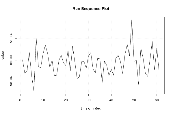
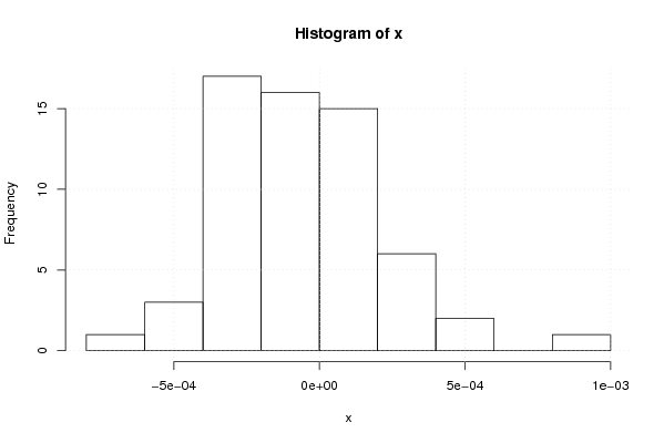
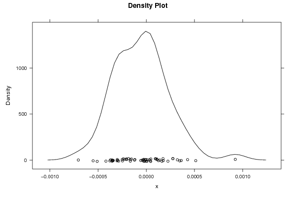
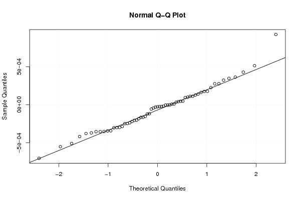
| Title produced by software | Univariate Explorative Data Analysis | ||||||||||||||||||||||||||||||||||||||||||||||||||||
| Date of computation | Thu, 10 Dec 2009 08:38:12 -0700 | ||||||||||||||||||||||||||||||||||||||||||||||||||||
| Cite this page as follows | Statistical Computations at FreeStatistics.org, Office for Research Development and Education, URL https://freestatistics.org/blog/index.php?v=date/2009/Dec/10/t12604599741hs2sr76kc1ctom.htm/, Retrieved Thu, 25 Apr 2024 20:21:21 +0000 | ||||||||||||||||||||||||||||||||||||||||||||||||||||
| Statistical Computations at FreeStatistics.org, Office for Research Development and Education, URL https://freestatistics.org/blog/index.php?pk=65501, Retrieved Thu, 25 Apr 2024 20:21:21 +0000 | |||||||||||||||||||||||||||||||||||||||||||||||||||||
| QR Codes: | |||||||||||||||||||||||||||||||||||||||||||||||||||||
|
| |||||||||||||||||||||||||||||||||||||||||||||||||||||
| Original text written by user: | |||||||||||||||||||||||||||||||||||||||||||||||||||||
| IsPrivate? | No (this computation is public) | ||||||||||||||||||||||||||||||||||||||||||||||||||||
| User-defined keywords | |||||||||||||||||||||||||||||||||||||||||||||||||||||
| Estimated Impact | 149 | ||||||||||||||||||||||||||||||||||||||||||||||||||||
Tree of Dependent Computations | |||||||||||||||||||||||||||||||||||||||||||||||||||||
| Family? (F = Feedback message, R = changed R code, M = changed R Module, P = changed Parameters, D = changed Data) | |||||||||||||||||||||||||||||||||||||||||||||||||||||
| - [Univariate Data Series] [Totaal levensmidd...] [2009-11-29 09:56:44] [757146c69eaf0537be37c7b0c18216d8] - RMPD [ARIMA Backward Selection] [arima backwards p...] [2009-12-10 13:12:43] [757146c69eaf0537be37c7b0c18216d8] - RMPD [Univariate Explorative Data Analysis] [Et assumpties na ...] [2009-12-10 15:38:12] [a931a0a30926b49d162330b43e89b999] [Current] - [Univariate Explorative Data Analysis] [Et assumpties na ...] [2009-12-21 15:08:38] [03c44f58d7d4de05d4cfabfda8c46d2c] - [Univariate Explorative Data Analysis] [et assumpties] [2009-12-21 15:35:48] [12f02da0296cb21dc23d82ae014a8b71] | |||||||||||||||||||||||||||||||||||||||||||||||||||||
| Feedback Forum | |||||||||||||||||||||||||||||||||||||||||||||||||||||
Post a new message | |||||||||||||||||||||||||||||||||||||||||||||||||||||
Dataset | |||||||||||||||||||||||||||||||||||||||||||||||||||||
| Dataseries X: | |||||||||||||||||||||||||||||||||||||||||||||||||||||
9.21658481064732e-06 -0.00029788936701127 -0.000237595445619398 0.000176386639516741 -0.000354517420077153 -0.000704448564633498 0.000513049322447122 -0.000153768338800356 -0.000165495788075780 0.000140072526121174 0.000346620687208592 0.000161916908058288 -0.000165099254299721 -1.69432824053433e-06 -0.000354149939969856 -0.000342774975550734 -4.96908925173395e-06 0.000111232688614015 -5.71770531287065e-05 -0.000121692129730065 0.000224672210051711 -0.000246864010604340 0.000322726843768265 -4.30529292240296e-05 -0.000418419406504748 -0.000378004975610374 -3.24021390863647e-05 -2.7363752224343e-05 -0.000183622849538695 9.90770631009303e-05 0.000173737572911515 -0.000202839888158976 -0.000286608152931299 4.11099519259386e-05 3.30589617581101e-05 -0.00050937217008082 -1.86226730255005e-05 -0.000118364395817495 -0.000351397442503670 -0.000205285906638802 -0.000344501241171445 4.54893857804128e-05 0.000109739140624292 -2.35892220696581e-05 -0.000303095753286898 0.000127032893461342 0.000362429017832127 9.35340989467158e-05 0.00092306316611607 -2.51463122583867e-05 -4.81959851185288e-06 -0.000551396477544085 0.000275472153350846 4.66854128330299e-05 -0.000300923258584334 -0.000370178149715601 7.01982462032013e-06 0.00042811187175734 -0.000220158172407577 0.000276271760846798 -0.000249130118572832 | |||||||||||||||||||||||||||||||||||||||||||||||||||||
Tables (Output of Computation) | |||||||||||||||||||||||||||||||||||||||||||||||||||||
| |||||||||||||||||||||||||||||||||||||||||||||||||||||
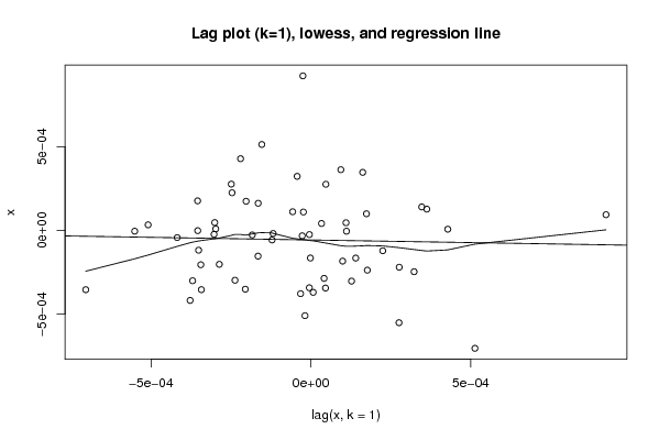
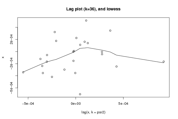
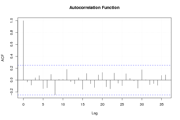
Figures (Output of Computation) | |||||||||||||||||||||||||||||||||||||||||||||||||||||
Input Parameters & R Code | |||||||||||||||||||||||||||||||||||||||||||||||||||||
| Parameters (Session): | |||||||||||||||||||||||||||||||||||||||||||||||||||||
| par1 = 0 ; par2 = 36 ; | |||||||||||||||||||||||||||||||||||||||||||||||||||||
| Parameters (R input): | |||||||||||||||||||||||||||||||||||||||||||||||||||||
| par1 = 0 ; par2 = 36 ; | |||||||||||||||||||||||||||||||||||||||||||||||||||||
| R code (references can be found in the software module): | |||||||||||||||||||||||||||||||||||||||||||||||||||||
par1 <- as.numeric(par1) | |||||||||||||||||||||||||||||||||||||||||||||||||||||