Free Statistics
of Irreproducible Research!
Description of Statistical Computation | |||||||||||||||||||||||||||||||||||||||||||||
|---|---|---|---|---|---|---|---|---|---|---|---|---|---|---|---|---|---|---|---|---|---|---|---|---|---|---|---|---|---|---|---|---|---|---|---|---|---|---|---|---|---|---|---|---|---|
| Author's title | |||||||||||||||||||||||||||||||||||||||||||||
| Author | *The author of this computation has been verified* | ||||||||||||||||||||||||||||||||||||||||||||
| R Software Module | rwasp_bidensity.wasp | ||||||||||||||||||||||||||||||||||||||||||||
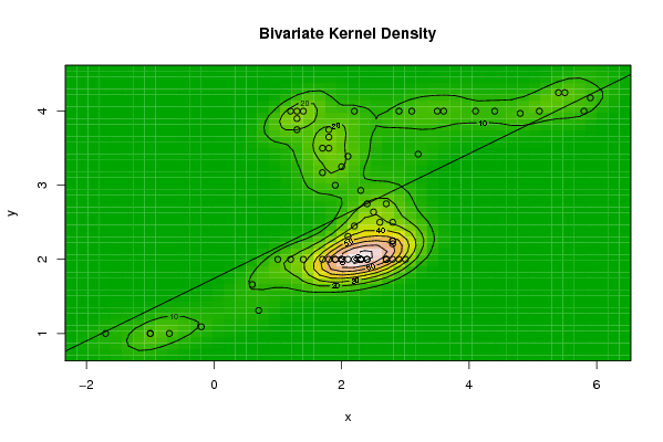
| Title produced by software | Bivariate Kernel Density Estimation | ||||||||||||||||||||||||||||||||||||||||||||
| Date of computation | Mon, 09 Nov 2009 01:32:40 -0700 | ||||||||||||||||||||||||||||||||||||||||||||
| Cite this page as follows | Statistical Computations at FreeStatistics.org, Office for Research Development and Education, URL https://freestatistics.org/blog/index.php?v=date/2009/Nov/09/t1257755725v6naaop1dk4pp7l.htm/, Retrieved Wed, 24 Apr 2024 11:32:42 +0000 | ||||||||||||||||||||||||||||||||||||||||||||
| Statistical Computations at FreeStatistics.org, Office for Research Development and Education, URL https://freestatistics.org/blog/index.php?pk=54658, Retrieved Wed, 24 Apr 2024 11:32:42 +0000 | |||||||||||||||||||||||||||||||||||||||||||||
| QR Codes: | |||||||||||||||||||||||||||||||||||||||||||||
|
| |||||||||||||||||||||||||||||||||||||||||||||
| Original text written by user: | |||||||||||||||||||||||||||||||||||||||||||||
| IsPrivate? | No (this computation is public) | ||||||||||||||||||||||||||||||||||||||||||||
| User-defined keywords | |||||||||||||||||||||||||||||||||||||||||||||
| Estimated Impact | 227 | ||||||||||||||||||||||||||||||||||||||||||||
Tree of Dependent Computations | |||||||||||||||||||||||||||||||||||||||||||||
| Family? (F = Feedback message, R = changed R code, M = changed R Module, P = changed Parameters, D = changed Data) | |||||||||||||||||||||||||||||||||||||||||||||
| - [Bivariate Kernel Density Estimation] [3/11/2009] [2009-11-02 21:54:51] [b98453cac15ba1066b407e146608df68] - PD [Bivariate Kernel Density Estimation] [] [2009-11-09 08:32:40] [fbab597368601c68e80be601720d8ff9] [Current] | |||||||||||||||||||||||||||||||||||||||||||||
| Feedback Forum | |||||||||||||||||||||||||||||||||||||||||||||
Post a new message | |||||||||||||||||||||||||||||||||||||||||||||
Dataset | |||||||||||||||||||||||||||||||||||||||||||||
| Dataseries X: | |||||||||||||||||||||||||||||||||||||||||||||
1,4 1,2 1 1,7 2,4 2 2,1 2 1,8 2,7 2,3 1,9 2 2,3 2,8 2,4 2,3 2,7 2,7 2,9 3 2,2 2,3 2,8 2,8 2,8 2,2 2,6 2,8 2,5 2,4 2,3 1,9 1,7 2 2,1 1,7 1,8 1,8 1,8 1,3 1,3 1,3 1,2 1,4 2,2 2,9 3,1 3,5 3,6 4,4 4,1 5,1 5,8 5,9 5,4 5,5 4,8 3,2 2,7 2,1 1,9 0,6 0,7 -0,2 -1 -1,7 -0,7 -1 | |||||||||||||||||||||||||||||||||||||||||||||
| Dataseries Y: | |||||||||||||||||||||||||||||||||||||||||||||
2 2 2 2 2 2 2 2 2 2 2 2 2 2 2 2 2 2 2 2 2 2 2 2,21 2,25 2,25 2,45 2,5 2,5 2,64 2,75 2,93 3 3,17 3,25 3,39 3,5 3,5 3,65 3,75 3,75 3,9 4 4 4 4 4 4 4 4 4 4 4 4 4,18 4,25 4,25 3,97 3,42 2,75 2,31 2 1,66 1,31 1,09 1 1 1 1 | |||||||||||||||||||||||||||||||||||||||||||||
Tables (Output of Computation) | |||||||||||||||||||||||||||||||||||||||||||||
| |||||||||||||||||||||||||||||||||||||||||||||
Figures (Output of Computation) | |||||||||||||||||||||||||||||||||||||||||||||
Input Parameters & R Code | |||||||||||||||||||||||||||||||||||||||||||||
| Parameters (Session): | |||||||||||||||||||||||||||||||||||||||||||||
| par1 = 50 ; par2 = 50 ; par3 = 0 ; par4 = 0 ; par5 = 0 ; par6 = Y ; par7 = Y ; | |||||||||||||||||||||||||||||||||||||||||||||
| Parameters (R input): | |||||||||||||||||||||||||||||||||||||||||||||
| par1 = 50 ; par2 = 50 ; par3 = 0 ; par4 = 0 ; par5 = 0 ; par6 = Y ; par7 = Y ; | |||||||||||||||||||||||||||||||||||||||||||||
| R code (references can be found in the software module): | |||||||||||||||||||||||||||||||||||||||||||||
par1 <- as(par1,'numeric') | |||||||||||||||||||||||||||||||||||||||||||||