Free Statistics
of Irreproducible Research!
Description of Statistical Computation | |||||||||||||||||||||
|---|---|---|---|---|---|---|---|---|---|---|---|---|---|---|---|---|---|---|---|---|---|
| Author's title | |||||||||||||||||||||
| Author | *The author of this computation has been verified* | ||||||||||||||||||||
| R Software Module | rwasp_meanplot.wasp | ||||||||||||||||||||
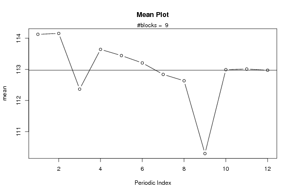
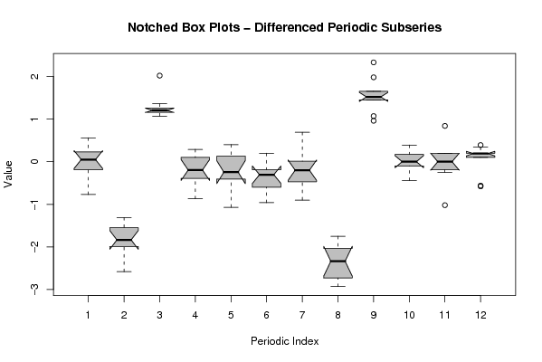
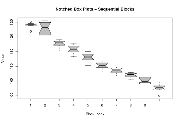
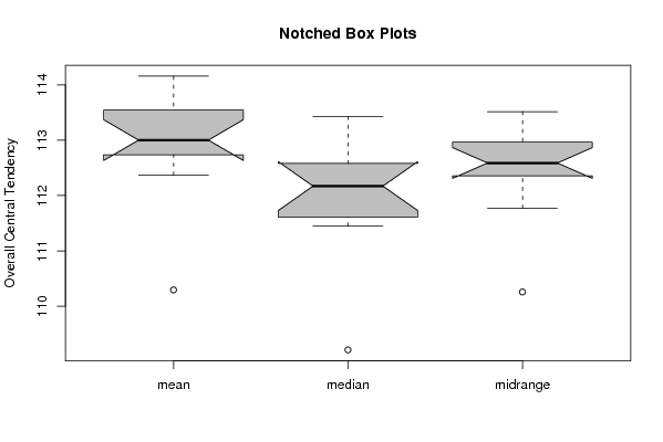
| Title produced by software | Mean Plot | ||||||||||||||||||||
| Date of computation | Mon, 09 Nov 2009 05:26:45 -0700 | ||||||||||||||||||||
| Cite this page as follows | Statistical Computations at FreeStatistics.org, Office for Research Development and Education, URL https://freestatistics.org/blog/index.php?v=date/2009/Nov/09/t1257769737vq7t942obyt5svj.htm/, Retrieved Tue, 23 Apr 2024 23:42:13 +0000 | ||||||||||||||||||||
| Statistical Computations at FreeStatistics.org, Office for Research Development and Education, URL https://freestatistics.org/blog/index.php?pk=54766, Retrieved Tue, 23 Apr 2024 23:42:13 +0000 | |||||||||||||||||||||
| QR Codes: | |||||||||||||||||||||
|
| |||||||||||||||||||||
| Original text written by user: | |||||||||||||||||||||
| IsPrivate? | No (this computation is public) | ||||||||||||||||||||
| User-defined keywords | |||||||||||||||||||||
| Estimated Impact | 202 | ||||||||||||||||||||
Tree of Dependent Computations | |||||||||||||||||||||
| Family? (F = Feedback message, R = changed R code, M = changed R Module, P = changed Parameters, D = changed Data) | |||||||||||||||||||||
| - [Mean Plot] [3/11/2009] [2009-11-02 22:07:54] [b98453cac15ba1066b407e146608df68] - PD [Mean Plot] [Mean Plot icp] [2009-11-09 12:26:45] [4f297b039e1043ebee7ff7a83b1eaaaa] [Current] | |||||||||||||||||||||
| Feedback Forum | |||||||||||||||||||||
Post a new message | |||||||||||||||||||||
Dataset | |||||||||||||||||||||
| Dataseries X: | |||||||||||||||||||||
124.06 124.58 122.00 124.02 124.16 124.29 123.93 124.62 121.81 124.14 124.31 125.15 125.35 125.48 124.17 125.33 124.46 123.39 123.14 122.24 119.31 120.87 120.43 119.41 118.85 119.08 117.25 118.51 118.42 118.56 117.97 117.98 115.25 117.23 117.08 116.83 117.17 117.73 115.74 116.99 116.90 116.49 115.84 115.92 113.32 114.84 114.75 114.84 115.03 115.03 112.99 114.15 113.77 113.57 113.38 112.71 110.27 111.73 112.12 112.31 111.73 111.83 109.99 111.15 111.25 110.87 110.27 110.18 108.15 109.60 109.60 109.41 109.80 109.60 107.76 109.02 108.62 109.02 109.22 108.92 106.69 107.76 107.66 107.85 107.95 107.85 106.30 107.37 107.66 107.46 107.37 107.18 105.43 106.39 106.50 106.50 106.69 106.50 105.14 106.50 106.20 105.72 104.76 104.55 102.71 104.36 104.65 104.46 104.65 103.88 102.32 103.39 103.00 102.71 102.51 102.04 100.00 | |||||||||||||||||||||
Tables (Output of Computation) | |||||||||||||||||||||
| |||||||||||||||||||||
Figures (Output of Computation) | |||||||||||||||||||||
Input Parameters & R Code | |||||||||||||||||||||
| Parameters (Session): | |||||||||||||||||||||
| par1 = 12 ; | |||||||||||||||||||||
| Parameters (R input): | |||||||||||||||||||||
| par1 = 12 ; | |||||||||||||||||||||
| R code (references can be found in the software module): | |||||||||||||||||||||
par1 <- as.numeric(par1) | |||||||||||||||||||||