Free Statistics
of Irreproducible Research!
Description of Statistical Computation | |||||||||||||||||||||||||||||||||||||||||||||
|---|---|---|---|---|---|---|---|---|---|---|---|---|---|---|---|---|---|---|---|---|---|---|---|---|---|---|---|---|---|---|---|---|---|---|---|---|---|---|---|---|---|---|---|---|---|
| Author's title | |||||||||||||||||||||||||||||||||||||||||||||
| Author | *The author of this computation has been verified* | ||||||||||||||||||||||||||||||||||||||||||||
| R Software Module | rwasp_boxcoxlin.wasp | ||||||||||||||||||||||||||||||||||||||||||||
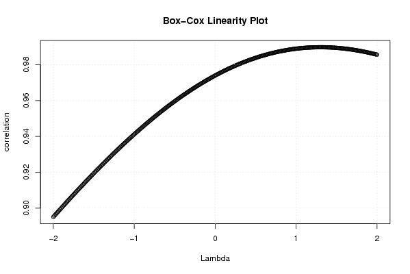
| Title produced by software | Box-Cox Linearity Plot | ||||||||||||||||||||||||||||||||||||||||||||
| Date of computation | Mon, 09 Nov 2009 14:08:36 -0700 | ||||||||||||||||||||||||||||||||||||||||||||
| Cite this page as follows | Statistical Computations at FreeStatistics.org, Office for Research Development and Education, URL https://freestatistics.org/blog/index.php?v=date/2009/Nov/09/t1257801187qaf7qwns60y5w56.htm/, Retrieved Sat, 20 Apr 2024 06:00:54 +0000 | ||||||||||||||||||||||||||||||||||||||||||||
| Statistical Computations at FreeStatistics.org, Office for Research Development and Education, URL https://freestatistics.org/blog/index.php?pk=55056, Retrieved Sat, 20 Apr 2024 06:00:54 +0000 | |||||||||||||||||||||||||||||||||||||||||||||
| QR Codes: | |||||||||||||||||||||||||||||||||||||||||||||
|
| |||||||||||||||||||||||||||||||||||||||||||||
| Original text written by user: | |||||||||||||||||||||||||||||||||||||||||||||
| IsPrivate? | No (this computation is public) | ||||||||||||||||||||||||||||||||||||||||||||
| User-defined keywords | |||||||||||||||||||||||||||||||||||||||||||||
| Estimated Impact | 197 | ||||||||||||||||||||||||||||||||||||||||||||
Tree of Dependent Computations | |||||||||||||||||||||||||||||||||||||||||||||
| Family? (F = Feedback message, R = changed R code, M = changed R Module, P = changed Parameters, D = changed Data) | |||||||||||||||||||||||||||||||||||||||||||||
| - [Partial Correlation] [3/11/2009] [2009-11-02 21:44:54] [b98453cac15ba1066b407e146608df68] - RM D [Box-Cox Linearity Plot] [WS6 box cox linea...] [2009-11-09 21:08:36] [557d56ec4b06cd0135c259898de8ce95] [Current] | |||||||||||||||||||||||||||||||||||||||||||||
| Feedback Forum | |||||||||||||||||||||||||||||||||||||||||||||
Post a new message | |||||||||||||||||||||||||||||||||||||||||||||
Dataset | |||||||||||||||||||||||||||||||||||||||||||||
| Dataseries X: | |||||||||||||||||||||||||||||||||||||||||||||
9904,642857 13710,15385 13747,69231 14517 15185,81818 11422,28571 13819,66667 12749 16217 13238 12391 14780,09091 10815,42857 14770,84615 11831 11931,3125 10611,94118 15923,18182 11094,875 16209,53846 10100 12149,6875 11644,35294 9249,947368 8980,777778 10244,52632 12457,5625 13307,46667 10839,625 11827,625 10925,94118 10675,3 9297,3 10433,21053 12261,41176 10911,22222 9334,421053 11655,05882 11080 9840,142857 7448,916667 8362,6 8465,64 8220,923077 10432,86364 8537,4 8535,464286 7997,464286 6301,413793 7595,566667 7200,483871 6152,482759 6064,259259 7269,909091 6578,44 7708,26087 6401,153846 7042,043478 8296,409091 9613,333333 | |||||||||||||||||||||||||||||||||||||||||||||
| Dataseries Y: | |||||||||||||||||||||||||||||||||||||||||||||
10284,5 12792 12823,61538 13845,66667 15335,63636 11188,5 13633,25 12298,46667 15353,63636 12696,15385 12213,93333 13683,72727 11214,14286 13950,23077 11179,13333 11801,875 11188,82353 16456,27273 11110,0625 16530,69231 10038,41176 11681,25 11148,88235 8631 9386,444444 9764,736842 12043,75 12948,06667 10987,125 11648,3125 10633,35294 10219,3 9037,6 10296,31579 11705,41176 10681,94444 9362,947368 11306,35294 10984,45 10062,61905 8118,583333 8867,48 8346,72 8529,307692 10697,18182 8591,84 8695,607143 8125,571429 7009,758621 7883,466667 7527,645161 6763,758621 6682,333333 7855,681818 6738,88 7895,434783 6361,884615 6935,956522 8344,454545 9107,944444 | |||||||||||||||||||||||||||||||||||||||||||||
Tables (Output of Computation) | |||||||||||||||||||||||||||||||||||||||||||||
| |||||||||||||||||||||||||||||||||||||||||||||
Figures (Output of Computation) | |||||||||||||||||||||||||||||||||||||||||||||
Input Parameters & R Code | |||||||||||||||||||||||||||||||||||||||||||||
| Parameters (Session): | |||||||||||||||||||||||||||||||||||||||||||||
| Parameters (R input): | |||||||||||||||||||||||||||||||||||||||||||||
| R code (references can be found in the software module): | |||||||||||||||||||||||||||||||||||||||||||||
n <- length(x) | |||||||||||||||||||||||||||||||||||||||||||||