| Multiple Linear Regression - Estimated Regression Equation |
| Y[t] = + 20.2513189201664 + 0.425341901487542totid[t] -0.0455449630743466ndzcg[t] + 0.0436802973309247indc[t] + 0.188344373020551y1[t] + 0.163567515100477y2[t] -0.130967620439291`y3 `[t] + 0.296514116202145M1[t] -0.835837579481557M2[t] -3.76745489042413M3[t] -2.08061356471506M4[t] -1.12030986429559M5[t] -1.97031879592753M6[t] -1.21767349589456M7[t] -1.11620771659602M8[t] + 1.25633708049614M9[t] + 0.269097496660407M10[t] -0.08551092511179M11[t] -0.166442807258652t + e[t] |
| Multiple Linear Regression - Ordinary Least Squares | |||||
| Variable | Parameter | S.D. | T-STAT H0: parameter = 0 | 2-tail p-value | 1-tail p-value |
| (Intercept) | 20.2513189201664 | 23.268082 | 0.8703 | 0.391022 | 0.195511 |
| totid | 0.425341901487542 | 0.244499 | 1.7396 | 0.092173 | 0.046086 |
| ndzcg | -0.0455449630743466 | 0.268582 | -0.1696 | 0.866482 | 0.433241 |
| indc | 0.0436802973309247 | 0.104583 | 0.4177 | 0.67917 | 0.339585 |
| y1 | 0.188344373020551 | 0.189551 | 0.9936 | 0.328348 | 0.164174 |
| y2 | 0.163567515100477 | 0.16883 | 0.9688 | 0.340378 | 0.170189 |
| `y3 ` | -0.130967620439291 | 0.163436 | -0.8013 | 0.429237 | 0.214619 |
| M1 | 0.296514116202145 | 2.127164 | 0.1394 | 0.89007 | 0.445035 |
| M2 | -0.835837579481557 | 2.415932 | -0.346 | 0.731781 | 0.36589 |
| M3 | -3.76745489042413 | 2.405121 | -1.5664 | 0.127737 | 0.063868 |
| M4 | -2.08061356471506 | 2.526785 | -0.8234 | 0.416765 | 0.208383 |
| M5 | -1.12030986429559 | 2.680751 | -0.4179 | 0.67899 | 0.339495 |
| M6 | -1.97031879592753 | 2.718052 | -0.7249 | 0.474129 | 0.237065 |
| M7 | -1.21767349589456 | 2.517465 | -0.4837 | 0.632118 | 0.316059 |
| M8 | -1.11620771659602 | 2.409731 | -0.4632 | 0.646558 | 0.323279 |
| M9 | 1.25633708049614 | 2.385667 | 0.5266 | 0.602331 | 0.301165 |
| M10 | 0.269097496660407 | 2.362987 | 0.1139 | 0.910091 | 0.455046 |
| M11 | -0.08551092511179 | 2.259958 | -0.0378 | 0.970068 | 0.485034 |
| t | -0.166442807258652 | 0.077479 | -2.1482 | 0.039892 | 0.019946 |
| Multiple Linear Regression - Regression Statistics | |
| Multiple R | 0.90975669067051 |
| R-squared | 0.827657236219756 |
| Adjusted R-squared | 0.72425157795161 |
| F-TEST (value) | 8.00398401868412 |
| F-TEST (DF numerator) | 18 |
| F-TEST (DF denominator) | 30 |
| p-value | 4.22611395878292e-07 |
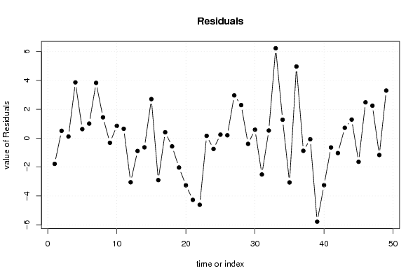
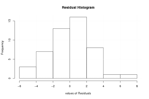
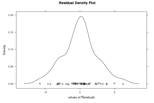
| Multiple Linear Regression - Residual Statistics | |
| Residual Standard Deviation | 3.10793514765004 |
| Sum Squared Residuals | 289.777826459955 |
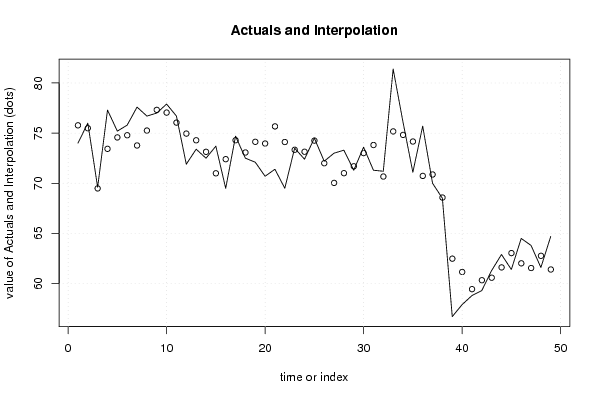
| Multiple Linear Regression - Actuals, Interpolation, and Residuals | |||
| Time or Index | Actuals | Interpolation Forecast | Residuals Prediction Error |
| 1 | 74 | 75.7790253566907 | -1.7790253566907 |
| 2 | 76 | 75.489644875326 | 0.510355124674 |
| 3 | 69.6 | 69.4873313009797 | 0.112668699020267 |
| 4 | 77.3 | 73.4345661294644 | 3.8654338705356 |
| 5 | 75.2 | 74.5720971867943 | 0.627902813205723 |
| 6 | 75.8 | 74.7897879567408 | 1.01021204325918 |
| 7 | 77.6 | 73.7690564989996 | 3.83094350100039 |
| 8 | 76.7 | 75.2556311242933 | 1.44436887570675 |
| 9 | 77 | 77.319662646084 | -0.319662646083947 |
| 10 | 77.9 | 77.0472393463657 | 0.852760653634317 |
| 11 | 76.7 | 76.0483913334632 | 0.651608666536769 |
| 12 | 71.9 | 74.9530612412628 | -3.05306124126283 |
| 13 | 73.4 | 74.287365418013 | -0.887365418013026 |
| 14 | 72.5 | 73.1341707360195 | -0.634170736019501 |
| 15 | 73.7 | 70.9931286521832 | 2.70687134781680 |
| 16 | 69.5 | 72.403824300446 | -2.90382430044602 |
| 17 | 74.7 | 74.2907497336154 | 0.409250266384581 |
| 18 | 72.5 | 73.06852201431 | -0.568522014310007 |
| 19 | 72.1 | 74.134010010568 | -2.03401001056808 |
| 20 | 70.7 | 73.9630595953059 | -3.26305959530586 |
| 21 | 71.4 | 75.6712787885589 | -4.27127878855884 |
| 22 | 69.5 | 74.1135899882116 | -4.61358998821163 |
| 23 | 73.5 | 73.3384810303127 | 0.161518969687286 |
| 24 | 72.4 | 73.1451494319208 | -0.745149431920782 |
| 25 | 74.5 | 74.2548286956975 | 0.245171304302463 |
| 26 | 72.2 | 72.0001066280042 | 0.199893371995791 |
| 27 | 73 | 70.036546237876 | 2.96345376212398 |
| 28 | 73.3 | 71.0070787401068 | 2.29292125989316 |
| 29 | 71.3 | 71.6943946969648 | -0.394394696964843 |
| 30 | 73.6 | 73.0088056803371 | 0.591194319662869 |
| 31 | 71.3 | 73.8152074810518 | -2.51520748105184 |
| 32 | 71.2 | 70.6700354480265 | 0.529964551973485 |
| 33 | 81.4 | 75.1719542420652 | 6.22804575793478 |
| 34 | 76.1 | 74.8211134934189 | 1.27888650658112 |
| 35 | 71.1 | 74.1638782899017 | -3.0638782899017 |
| 36 | 75.7 | 70.7356335169924 | 4.96436648300763 |
| 37 | 70 | 70.876052990832 | -0.876052990831986 |
| 38 | 68.5 | 68.5760777606503 | -0.0760777606502896 |
| 39 | 56.7 | 62.482993808961 | -5.78299380896104 |
| 40 | 57.9 | 61.1545308299827 | -3.25453082998274 |
| 41 | 58.8 | 59.4427583826255 | -0.64275838262546 |
| 42 | 59.3 | 60.332884348612 | -1.03288434861204 |
| 43 | 61.3 | 60.5817260093805 | 0.718273990619535 |
| 44 | 62.9 | 61.6112738323744 | 1.28872616762563 |
| 45 | 61.4 | 63.037104323292 | -1.63710432329199 |
| 46 | 64.5 | 62.0180571720038 | 2.48194282799619 |
| 47 | 63.8 | 61.5492493463223 | 2.25075065367765 |
| 48 | 61.6 | 62.766155809824 | -1.16615580982402 |
| 49 | 64.7 | 61.4027275387668 | 3.29727246123325 |
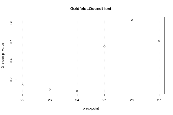
| Goldfeld-Quandt test for Heteroskedasticity | |||
| p-values | Alternative Hypothesis | ||
| breakpoint index | greater | 2-sided | less |
| 22 | 0.0716374951492726 | 0.143274990298545 | 0.928362504850727 |
| 23 | 0.0489277650497474 | 0.0978555300994948 | 0.951072234950253 |
| 24 | 0.0409123541930088 | 0.0818247083860176 | 0.959087645806991 |
| 25 | 0.276858783762207 | 0.553717567524414 | 0.723141216237793 |
| 26 | 0.41717679278587 | 0.83435358557174 | 0.58282320721413 |
| 27 | 0.306602647819216 | 0.613205295638432 | 0.693397352180784 |
| Meta Analysis of Goldfeld-Quandt test for Heteroskedasticity | |||
| Description | # significant tests | % significant tests | OK/NOK |
| 1% type I error level | 0 | 0 | OK |
| 5% type I error level | 0 | 0 | OK |
| 10% type I error level | 2 | 0.333333333333333 | NOK |