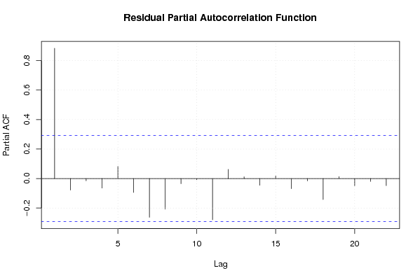
| Multiple Linear Regression - Estimated Regression Equation |
| Ktot[t] = + 105.065867086302 -0.0486175142110252Vmtot[t] + 0.0380062117884138M1[t] -0.201647603739741M2[t] -0.179270889616640M3[t] -0.173762836424627M4[t] -0.158416651952784M5[t] -0.21222427121419M6[t] -0.26500251046336M7[t] -0.283688585939234M8[t] -0.237265212191018M9[t] -0.0543179461956548M10[t] + 0.0224500909672896M11[t] + 0.0767557745848375t + e[t] |
| Multiple Linear Regression - Ordinary Least Squares | |||||
| Variable | Parameter | S.D. | T-STAT H0: parameter = 0 | 2-tail p-value | 1-tail p-value |
| (Intercept) | 105.065867086302 | 2.265547 | 46.3755 | 0 | 0 |
| Vmtot | -0.0486175142110252 | 0.022122 | -2.1977 | 0.035565 | 0.017782 |
| M1 | 0.0380062117884138 | 0.156693 | 0.2426 | 0.80995 | 0.404975 |
| M2 | -0.201647603739741 | 0.156255 | -1.2905 | 0.206418 | 0.103209 |
| M3 | -0.179270889616640 | 0.155919 | -1.1498 | 0.259031 | 0.129516 |
| M4 | -0.173762836424627 | 0.156724 | -1.1087 | 0.276079 | 0.13804 |
| M5 | -0.158416651952784 | 0.156277 | -1.0137 | 0.318577 | 0.159289 |
| M6 | -0.21222427121419 | 0.155908 | -1.3612 | 0.18326 | 0.09163 |
| M7 | -0.26500251046336 | 0.156041 | -1.6983 | 0.09947 | 0.049735 |
| M8 | -0.283688585939234 | 0.158481 | -1.79 | 0.083219 | 0.04161 |
| M9 | -0.237265212191018 | 0.158833 | -1.4938 | 0.145337 | 0.072669 |
| M10 | -0.0543179461956548 | 0.166577 | -0.3261 | 0.746553 | 0.373276 |
| M11 | 0.0224500909672896 | 0.166715 | 0.1347 | 0.89375 | 0.446875 |
| t | 0.0767557745848375 | 0.008868 | 8.6558 | 0 | 0 |
| Multiple Linear Regression - Regression Statistics | |
| Multiple R | 0.975852123483842 |
| R-squared | 0.952287366907923 |
| Adjusted R-squared | 0.932278843353181 |
| F-TEST (value) | 47.5940848060344 |
| F-TEST (DF numerator) | 13 |
| F-TEST (DF denominator) | 31 |
| p-value | 1.11022302462516e-16 |
| Multiple Linear Regression - Residual Statistics | |
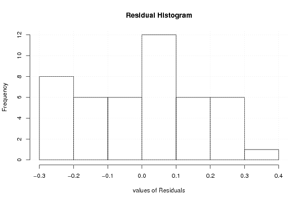
| Residual Standard Deviation | 0.20392119736432 |
| Sum Squared Residuals | 1.28909949676944 |
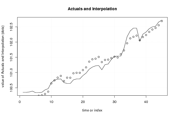
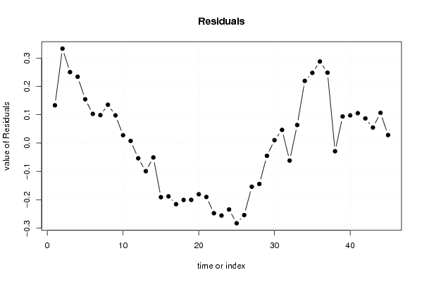
| Multiple Linear Regression - Actuals, Interpolation, and Residuals | |||
| Time or Index | Actuals | Interpolation Forecast | Residuals Prediction Error |
| 1 | 100.35 | 100.216780871730 | 0.133219128270414 |
| 2 | 100.35 | 100.016933519986 | 0.333066480014129 |
| 3 | 100.36 | 100.109745731846 | 0.250254268153627 |
| 4 | 100.39 | 100.156032599107 | 0.233967400892937 |
| 5 | 100.34 | 100.185417964832 | 0.154582035168482 |
| 6 | 100.34 | 100.237050453539 | 0.102949546460546 |
| 7 | 100.35 | 100.251304486033 | 0.0986955139670732 |
| 8 | 100.43 | 100.294788930879 | 0.135211069121431 |
| 9 | 100.47 | 100.372267615853 | 0.0977323841467326 |
| 10 | 100.67 | 100.642180334418 | 0.0278196655822193 |
| 11 | 100.75 | 100.742224880533 | 0.00777511946656353 |
| 12 | 100.78 | 100.833479874951 | -0.0534798749513622 |
| 13 | 100.79 | 100.888928493987 | -0.0989284939871578 |
| 14 | 100.67 | 100.720682526481 | -0.0506825264806321 |
| 15 | 100.64 | 100.830510868315 | -0.190510868314998 |
| 16 | 100.64 | 100.827694046223 | -0.187694046222554 |
| 17 | 100.76 | 100.975219971480 | -0.215219971479798 |
| 18 | 100.79 | 100.990389324529 | -0.200389324529465 |
| 19 | 100.79 | 100.990058102760 | -0.20005810275962 |
| 20 | 100.9 | 101.080215361248 | -0.18021536124786 |
| 21 | 100.98 | 101.169848424775 | -0.189848424775308 |
| 22 | 101.11 | 101.357111369181 | -0.247111369181086 |
| 23 | 101.18 | 101.435278033902 | -0.255278033901771 |
| 24 | 101.22 | 101.454092932145 | -0.234092932145278 |
| 25 | 101.23 | 101.512458602034 | -0.282458602033736 |
| 26 | 101.09 | 101.343726459385 | -0.253726459385096 |
| 27 | 101.26 | 101.413688439566 | -0.153688439566418 |
| 28 | 101.28 | 101.423998346311 | -0.143998346310954 |
| 29 | 101.43 | 101.474775418288 | -0.0447754182882581 |
| 30 | 101.53 | 101.519601455007 | 0.0103985449933431 |
| 31 | 101.54 | 101.493502950705 | 0.0464970492950365 |
| 32 | 101.54 | 101.601648689451 | -0.0616486894512825 |
| 33 | 101.79 | 101.726286363211 | 0.0637136367893329 |
| 34 | 102.18 | 101.960708296401 | 0.219291703598866 |
| 35 | 102.37 | 102.122497085565 | 0.247502914435208 |
| 36 | 102.46 | 102.172427192903 | 0.287572807096641 |
| 37 | 102.46 | 102.211832032250 | 0.248167967750479 |
| 38 | 102.03 | 102.058657494148 | -0.0286574941484009 |
| 39 | 102.26 | 102.166054960272 | 0.0939450397277893 |
| 40 | 102.33 | 102.232275008359 | 0.0977249916405709 |
| 41 | 102.44 | 102.334586645400 | 0.105413354599575 |
| 42 | 102.5 | 102.412958766924 | 0.0870412330755766 |
| 43 | 102.52 | 102.465134460502 | 0.0548655394975103 |
| 44 | 102.66 | 102.553347018422 | 0.106652981577712 |
| 45 | 102.72 | 102.691597596161 | 0.0284024038392427 |
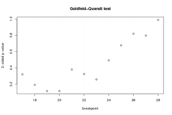
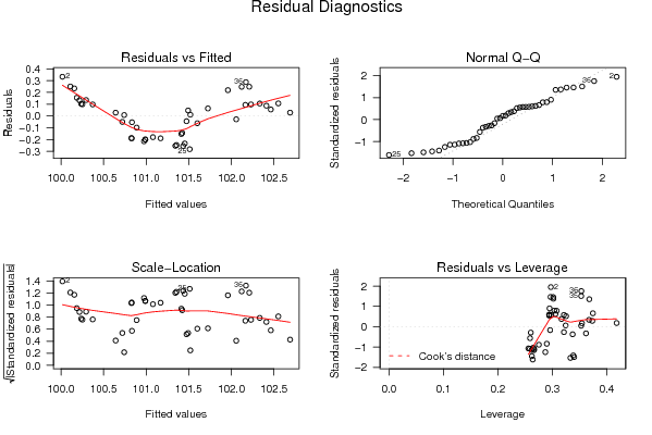
| Goldfeld-Quandt test for Heteroskedasticity | |||
| p-values | Alternative Hypothesis | ||
| breakpoint index | greater | 2-sided | less |
| 17 | 0.159889689320657 | 0.319779378641315 | 0.840110310679343 |
| 18 | 0.0955462955625386 | 0.191092591125077 | 0.904453704437461 |
| 19 | 0.0575885512366176 | 0.115177102473235 | 0.942411448763382 |
| 20 | 0.0577449473878358 | 0.115489894775672 | 0.942255052612164 |
| 21 | 0.189869690817305 | 0.37973938163461 | 0.810130309182695 |
| 22 | 0.162059918214418 | 0.324119836428836 | 0.837940081785582 |
| 23 | 0.129044152837192 | 0.258088305674385 | 0.870955847162808 |
| 24 | 0.246059484657333 | 0.492118969314666 | 0.753940515342667 |
| 25 | 0.66183617001887 | 0.676327659962259 | 0.338163829981129 |
| 26 | 0.590064563777703 | 0.819870872444595 | 0.409935436222297 |
| 27 | 0.601779357410566 | 0.796441285178867 | 0.398220642589434 |
| 28 | 0.495008936103683 | 0.990017872207366 | 0.504991063896317 |
| Meta Analysis of Goldfeld-Quandt test for Heteroskedasticity | |||
| Description | # significant tests | % significant tests | OK/NOK |
| 1% type I error level | 0 | 0 | OK |
| 5% type I error level | 0 | 0 | OK |
| 10% type I error level | 0 | 0 | OK |