Free Statistics
of Irreproducible Research!
Description of Statistical Computation | |||||||||||||||||||||||||||||||||||||||||||||||||||||||||||||||||||||||||||||||||||||||||||||||||||||||||||||||||||||||||||||||||||||||||||||||||||||||||||||||||||||||||||||||||||||||||||||||||||||||||
|---|---|---|---|---|---|---|---|---|---|---|---|---|---|---|---|---|---|---|---|---|---|---|---|---|---|---|---|---|---|---|---|---|---|---|---|---|---|---|---|---|---|---|---|---|---|---|---|---|---|---|---|---|---|---|---|---|---|---|---|---|---|---|---|---|---|---|---|---|---|---|---|---|---|---|---|---|---|---|---|---|---|---|---|---|---|---|---|---|---|---|---|---|---|---|---|---|---|---|---|---|---|---|---|---|---|---|---|---|---|---|---|---|---|---|---|---|---|---|---|---|---|---|---|---|---|---|---|---|---|---|---|---|---|---|---|---|---|---|---|---|---|---|---|---|---|---|---|---|---|---|---|---|---|---|---|---|---|---|---|---|---|---|---|---|---|---|---|---|---|---|---|---|---|---|---|---|---|---|---|---|---|---|---|---|---|---|---|---|---|---|---|---|---|---|---|---|---|---|---|---|---|
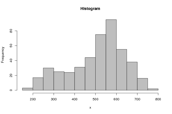
| Author's title | frequentietabel van maandelijks geproduceerde hoeveelheid ruw staal in Aust... | ||||||||||||||||||||||||||||||||||||||||||||||||||||||||||||||||||||||||||||||||||||||||||||||||||||||||||||||||||||||||||||||||||||||||||||||||||||||||||||||||||||||||||||||||||||||||||||||||||||||||
| Author | *Unverified author* | ||||||||||||||||||||||||||||||||||||||||||||||||||||||||||||||||||||||||||||||||||||||||||||||||||||||||||||||||||||||||||||||||||||||||||||||||||||||||||||||||||||||||||||||||||||||||||||||||||||||||
| R Software Module | rwasp_histogram.wasp | ||||||||||||||||||||||||||||||||||||||||||||||||||||||||||||||||||||||||||||||||||||||||||||||||||||||||||||||||||||||||||||||||||||||||||||||||||||||||||||||||||||||||||||||||||||||||||||||||||||||||
| Title produced by software | Histogram | ||||||||||||||||||||||||||||||||||||||||||||||||||||||||||||||||||||||||||||||||||||||||||||||||||||||||||||||||||||||||||||||||||||||||||||||||||||||||||||||||||||||||||||||||||||||||||||||||||||||||
| Date of computation | Wed, 10 Feb 2010 11:03:59 -0700 | ||||||||||||||||||||||||||||||||||||||||||||||||||||||||||||||||||||||||||||||||||||||||||||||||||||||||||||||||||||||||||||||||||||||||||||||||||||||||||||||||||||||||||||||||||||||||||||||||||||||||
| Cite this page as follows | Statistical Computations at FreeStatistics.org, Office for Research Development and Education, URL https://freestatistics.org/blog/index.php?v=date/2010/Feb/10/t1265825297v6rigopzl0uux6l.htm/, Retrieved Tue, 23 Apr 2024 11:35:52 +0000 | ||||||||||||||||||||||||||||||||||||||||||||||||||||||||||||||||||||||||||||||||||||||||||||||||||||||||||||||||||||||||||||||||||||||||||||||||||||||||||||||||||||||||||||||||||||||||||||||||||||||||
| Statistical Computations at FreeStatistics.org, Office for Research Development and Education, URL https://freestatistics.org/blog/index.php?pk=72979, Retrieved Tue, 23 Apr 2024 11:35:52 +0000 | |||||||||||||||||||||||||||||||||||||||||||||||||||||||||||||||||||||||||||||||||||||||||||||||||||||||||||||||||||||||||||||||||||||||||||||||||||||||||||||||||||||||||||||||||||||||||||||||||||||||||
| QR Codes: | |||||||||||||||||||||||||||||||||||||||||||||||||||||||||||||||||||||||||||||||||||||||||||||||||||||||||||||||||||||||||||||||||||||||||||||||||||||||||||||||||||||||||||||||||||||||||||||||||||||||||
|
| |||||||||||||||||||||||||||||||||||||||||||||||||||||||||||||||||||||||||||||||||||||||||||||||||||||||||||||||||||||||||||||||||||||||||||||||||||||||||||||||||||||||||||||||||||||||||||||||||||||||||
| Original text written by user: | |||||||||||||||||||||||||||||||||||||||||||||||||||||||||||||||||||||||||||||||||||||||||||||||||||||||||||||||||||||||||||||||||||||||||||||||||||||||||||||||||||||||||||||||||||||||||||||||||||||||||
| IsPrivate? | No (this computation is public) | ||||||||||||||||||||||||||||||||||||||||||||||||||||||||||||||||||||||||||||||||||||||||||||||||||||||||||||||||||||||||||||||||||||||||||||||||||||||||||||||||||||||||||||||||||||||||||||||||||||||||
| User-defined keywords | KDGP1W1 | ||||||||||||||||||||||||||||||||||||||||||||||||||||||||||||||||||||||||||||||||||||||||||||||||||||||||||||||||||||||||||||||||||||||||||||||||||||||||||||||||||||||||||||||||||||||||||||||||||||||||
| Estimated Impact | 133 | ||||||||||||||||||||||||||||||||||||||||||||||||||||||||||||||||||||||||||||||||||||||||||||||||||||||||||||||||||||||||||||||||||||||||||||||||||||||||||||||||||||||||||||||||||||||||||||||||||||||||
Tree of Dependent Computations | |||||||||||||||||||||||||||||||||||||||||||||||||||||||||||||||||||||||||||||||||||||||||||||||||||||||||||||||||||||||||||||||||||||||||||||||||||||||||||||||||||||||||||||||||||||||||||||||||||||||||
| Family? (F = Feedback message, R = changed R code, M = changed R Module, P = changed Parameters, D = changed Data) | |||||||||||||||||||||||||||||||||||||||||||||||||||||||||||||||||||||||||||||||||||||||||||||||||||||||||||||||||||||||||||||||||||||||||||||||||||||||||||||||||||||||||||||||||||||||||||||||||||||||||
| - [Histogram] [frequentietabel v...] [2010-02-10 18:03:59] [33936929259c41adeea2425316690930] [Current] | |||||||||||||||||||||||||||||||||||||||||||||||||||||||||||||||||||||||||||||||||||||||||||||||||||||||||||||||||||||||||||||||||||||||||||||||||||||||||||||||||||||||||||||||||||||||||||||||||||||||||
| Feedback Forum | |||||||||||||||||||||||||||||||||||||||||||||||||||||||||||||||||||||||||||||||||||||||||||||||||||||||||||||||||||||||||||||||||||||||||||||||||||||||||||||||||||||||||||||||||||||||||||||||||||||||||
Post a new message | |||||||||||||||||||||||||||||||||||||||||||||||||||||||||||||||||||||||||||||||||||||||||||||||||||||||||||||||||||||||||||||||||||||||||||||||||||||||||||||||||||||||||||||||||||||||||||||||||||||||||
Dataset | |||||||||||||||||||||||||||||||||||||||||||||||||||||||||||||||||||||||||||||||||||||||||||||||||||||||||||||||||||||||||||||||||||||||||||||||||||||||||||||||||||||||||||||||||||||||||||||||||||||||||
| Dataseries X: | |||||||||||||||||||||||||||||||||||||||||||||||||||||||||||||||||||||||||||||||||||||||||||||||||||||||||||||||||||||||||||||||||||||||||||||||||||||||||||||||||||||||||||||||||||||||||||||||||||||||||
196.9 192.1 201.8 186.9 218.0 214.4 227.5 204.1 225.8 223.7 244.7 243.9 257.3 234.5 251.4 243.8 247.4 245.3 262.5 270.0 259.9 262.2 244.9 249.3 268.2 231.2 264.3 252.7 275.5 261.5 275.5 272.3 268.6 270.4 267.7 275.0 272.6 248.6 279.4 270.5 292.8 297.8 296.8 290.9 282.8 312.8 303.2 301.4 289.8 279.6 302.2 299.1 319.7 310.9 315.2 338.5 315.6 321.2 318.5 342.7 261.4 287.0 331.5 326.9 338.6 337.0 358.4 344.5 345.7 344.1 317.4 354.5 345.2 314.1 352.5 361.2 365.9 332.5 364.0 359.1 345.6 366.9 370.2 359.9 366.6 336.3 368.5 374.2 384.3 358.9 407.7 433.3 404.7 392.7 409.7 416.5 414.3 404.3 421.4 372.6 404.7 420.2 438.4 449.1 445.8 413.8 420.5 442.3 438.9 394.5 416.8 402.9 424.5 432.3 484.1 492.7 496.3 471.9 491.2 512.9 482.4 407.9 448.5 431.1 498.8 497.1 517.1 487.7 512.5 550.1 532.5 524.1 515.7 461.0 529.3 467.4 559.8 536.5 531.9 546.5 547.4 536.1 482.8 551.0 532.9 484.1 554.8 537.0 558.0 511.4 502.9 558.6 545.1 574.3 542.2 600.0 588.6 524.4 618.5 580.9 557.2 571.2 597.5 601.7 558.9 600.9 601.0 615.7 578.1 495.9 526.8 522.1 605.1 574.4 609.7 580.7 565.1 590.7 571.5 601.3 567.3 467.9 588.9 579.4 502.6 568.7 616.0 586.2 575.5 599.9 568.2 516.0 493.4 496.8 529.9 491.7 543.2 490.8 554.7 625.7 605.0 645.2 645.2 611.8 600.3 549.8 635.5 617.7 643.5 485.7 689.5 692.0 677.3 704.7 668.6 717.8 689.8 640.4 675.2 528.1 538.0 527.2 655.6 650.6 623.7 748.4 727.4 750.5 678.9 659.5 691.9 639.8 663.8 572.9 592.5 734.8 696.1 589.2 662.9 661.2 672.1 583.7 705.5 631.0 733.3 674.9 695.5 634.1 630.6 635.2 554.1 623.9 679.3 565.6 564.1 637.2 650.8 602.7 587.5 619.2 616.5 637.9 557.9 594.0 668.7 603.3 674.5 573.4 706.0 693.7 627.5 550.7 592.3 660.2 597.3 641.0 663.6 595.9 638.4 665.4 671.4 637.0 685.7 705.8 704.8 734.4 674.2 748.6 763.4 658.0 627.5 528.9 488.3 575.5 735.6 685.3 613.6 629.5 634.7 652.6 728.3 634.3 690.7 676.3 675.4 595.6 712.4 735.8 544.4 567.0 510.0 564.0 630.7 496.7 660.9 601.2 655.2 591.6 606.1 560.7 368.3 371.6 413.9 413.9 389.0 399.2 429.8 395.6 472.0 486.0 525.0 396.0 511.0 525.0 492.0 517.0 525.0 474.0 539.0 468.0 543.0 532.0 565.0 535.0 534.0 546.0 494.0 552.0 511.0 451.0 537.0 494.0 549.0 544.0 598.0 583.0 582.0 589.0 578.0 561.0 592.0 504.0 545.0 547.0 585.0 562.0 520.0 581.0 590.0 562.0 548.0 567.0 542.0 473.0 531.0 462.0 479.0 533.0 552.0 547.0 562.0 524.0 479.0 445.0 406.0 475.0 589.0 495.0 484.0 536.0 555.0 565.0 564.0 573.0 569.0 588.0 546.0 508.0 560.0 558.0 516.0 549.0 595.0 586.0 597.0 592.0 538.0 590.0 576.0 451.0 538.0 555.0 532.0 530.0 553.0 626.0 601.0 573.0 569.0 562.0 468.0 483.0 460.0 411.0 458.0 455.0 600.0 605.0 545.0 549.0 415.0 568.0 577.0 517.0 558.0 518.0 489.0 502.0 569.0 540.0 550.0 557.0 542.0 542.0 582.0 525.0 584.0 562.0 639.0 613.0 604.0 613.0 625.0 654.0 638.0 | |||||||||||||||||||||||||||||||||||||||||||||||||||||||||||||||||||||||||||||||||||||||||||||||||||||||||||||||||||||||||||||||||||||||||||||||||||||||||||||||||||||||||||||||||||||||||||||||||||||||||
Tables (Output of Computation) | |||||||||||||||||||||||||||||||||||||||||||||||||||||||||||||||||||||||||||||||||||||||||||||||||||||||||||||||||||||||||||||||||||||||||||||||||||||||||||||||||||||||||||||||||||||||||||||||||||||||||
| |||||||||||||||||||||||||||||||||||||||||||||||||||||||||||||||||||||||||||||||||||||||||||||||||||||||||||||||||||||||||||||||||||||||||||||||||||||||||||||||||||||||||||||||||||||||||||||||||||||||||
Figures (Output of Computation) | |||||||||||||||||||||||||||||||||||||||||||||||||||||||||||||||||||||||||||||||||||||||||||||||||||||||||||||||||||||||||||||||||||||||||||||||||||||||||||||||||||||||||||||||||||||||||||||||||||||||||
Input Parameters & R Code | |||||||||||||||||||||||||||||||||||||||||||||||||||||||||||||||||||||||||||||||||||||||||||||||||||||||||||||||||||||||||||||||||||||||||||||||||||||||||||||||||||||||||||||||||||||||||||||||||||||||||
| Parameters (Session): | |||||||||||||||||||||||||||||||||||||||||||||||||||||||||||||||||||||||||||||||||||||||||||||||||||||||||||||||||||||||||||||||||||||||||||||||||||||||||||||||||||||||||||||||||||||||||||||||||||||||||
| par1 = Start of session ; par2 = Start of session ; par3 = Start of session ; par4 = Start of session ; par5 = Start of session ; par6 = Start of session ; par7 = Start of session ; par8 = Start of session ; par9 = Start of session ; par10 = Start of session ; par11 = Start of session ; par12 = Start of session ; par13 = Start of session ; par14 = Start of session ; par15 = Start of session ; par16 = Start of session ; par17 = Start of session ; par18 = Start of session ; par19 = Start of session ; par20 = Start of session ; | |||||||||||||||||||||||||||||||||||||||||||||||||||||||||||||||||||||||||||||||||||||||||||||||||||||||||||||||||||||||||||||||||||||||||||||||||||||||||||||||||||||||||||||||||||||||||||||||||||||||||
| Parameters (R input): | |||||||||||||||||||||||||||||||||||||||||||||||||||||||||||||||||||||||||||||||||||||||||||||||||||||||||||||||||||||||||||||||||||||||||||||||||||||||||||||||||||||||||||||||||||||||||||||||||||||||||
| par1 = ; par2 = grey ; par3 = FALSE ; par4 = Unknown ; | |||||||||||||||||||||||||||||||||||||||||||||||||||||||||||||||||||||||||||||||||||||||||||||||||||||||||||||||||||||||||||||||||||||||||||||||||||||||||||||||||||||||||||||||||||||||||||||||||||||||||
| R code (references can be found in the software module): | |||||||||||||||||||||||||||||||||||||||||||||||||||||||||||||||||||||||||||||||||||||||||||||||||||||||||||||||||||||||||||||||||||||||||||||||||||||||||||||||||||||||||||||||||||||||||||||||||||||||||
par1 <- as.numeric(par1) | |||||||||||||||||||||||||||||||||||||||||||||||||||||||||||||||||||||||||||||||||||||||||||||||||||||||||||||||||||||||||||||||||||||||||||||||||||||||||||||||||||||||||||||||||||||||||||||||||||||||||