Repository of Reproducible Computations

Free Statistics

of Irreproducible Research!

Author's title

Author

*Unverified author*

R Software Module

rwasp_autocorrelation.wasp

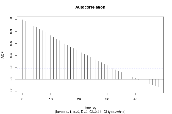
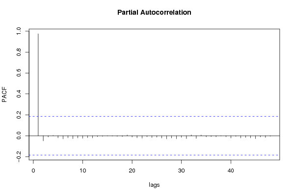
Title produced by software

(Partial) Autocorrelation Function

Date of computation

Mon, 03 May 2010 16:09:16 +0000

Cite this page as follows

Statistical Computations at FreeStatistics.org, Office for Research Development and Education, URL https://freestatistics.org/blog/index.php?v=date/2010/May/03/t1272903071fgsf687p4iebg8n.htm/, Retrieved Fri, 19 Apr 2024 13:18:46 +0000

Statistical Computations at FreeStatistics.org, Office for Research Development and Education, URL https://freestatistics.org/blog/index.php?pk=75245, Retrieved Fri, 19 Apr 2024 13:18:46 +0000

QR Codes:

Paste this QR Code to cite your computation.

Original text written by user:

IsPrivate?

No (this computation is public)

User-defined keywords

KDGP2W21

Estimated Impact

116

Family? (F = Feedback message, R = changed R code, M = changed R Module, P = changed Parameters, D = changed Data)

-       [(Partial) Autocorrelation Function] [Melino Olivini] [2010-05-03 16:09:16] [2156736b6f7843cba1ea73b621b47743] [Current]

Feedback Forum

Post a new message

Dataseries X:

Download CSV

Histogram

Boxplots

Summary of computational transaction
Raw Input	view raw input (R code)
Raw Output	view raw output of R engine
Computing time	2 seconds
R Server	'Sir Ronald Aylmer Fisher' @ 193.190.124.24

\begin{tabular}{lllllllll}
\hline
Summary of computational transaction \tabularnewline
Raw Input & view raw input (R code)  \tabularnewline
Raw Output & view raw output of R engine  \tabularnewline
Computing time & 2 seconds \tabularnewline
R Server & 'Sir Ronald Aylmer Fisher' @ 193.190.124.24 \tabularnewline
\hline
\end{tabular}
%Source: https://freestatistics.org/blog/index.php?pk=75245&T=0

[TABLE]
[ROW][C]Summary of computational transaction[/C][/ROW]
[ROW][C]Raw Input[/C][C]view raw input (R code) [/C][/ROW]
[ROW][C]Raw Output[/C][C]view raw output of R engine [/C][/ROW]
[ROW][C]Computing time[/C][C]2 seconds[/C][/ROW]
[ROW][C]R Server[/C][C]'Sir Ronald Aylmer Fisher' @ 193.190.124.24[/C][/ROW]
[/TABLE]
Source: https://freestatistics.org/blog/index.php?pk=75245&T=0

Globally Unique Identifier (entire table): ba.freestatistics.org/blog/index.php?pk=75245&T=0

As an alternative you can also use a QR Code:

The GUIDs for individual cells are displayed in the table below:

Summary of computational transaction
Raw Input	view raw input (R code)
Raw Output	view raw output of R engine
Computing time	2 seconds
R Server	'Sir Ronald Aylmer Fisher' @ 193.190.124.24

Autocorrelation Function
Time lag k	ACF(k)	T-STAT	P-value
1	0.975298	10.3216	0
2	0.948826	10.0414	0
3	0.922394	9.7617	0
4	0.896766	9.4905	0
5	0.870919	9.2169	0
6	0.844295	8.9352	0
7	0.817382	8.6504	0
8	0.789816	8.3586	0
9	0.761987	8.0641	0
10	0.733761	7.7654	0
11	0.705433	7.4656	0
12	0.676927	7.1639	0
13	0.648772	6.866	0
14	0.621197	6.5741	0
15	0.594361	6.2901	0
16	0.568234	6.0136	0
17	0.542655	5.7429	0
18	0.517551	5.4772	0
19	0.493632	5.2241	0
20	0.469992	4.9739	1e-06
21	0.446218	4.7223	3e-06
22	0.422151	4.4676	9e-06
23	0.398479	4.2171	2.5e-05
24	0.374899	3.9676	6.4e-05
25	0.35156	3.7206	0.000156
26	0.328039	3.4716	0.000368
27	0.303963	3.2168	0.000847
28	0.279728	2.9604	0.001876
29	0.255029	2.699	0.004017
30	0.230555	2.44	0.008129
31	0.205739	2.1773	0.015777
32	0.182262	1.9289	0.028139
33	0.15855	1.6779	0.048074
34	0.13615	1.4409	0.076205
35	0.114235	1.209	0.114614
36	0.092887	0.983	0.163858
37	0.072023	0.7622	0.223767
38	0.051998	0.5503	0.291607
39	0.032573	0.3447	0.365475
40	0.013143	0.1391	0.444816
41	-0.00552	-0.0584	0.476758
42	-0.024124	-0.2553	0.399479
43	-0.042428	-0.449	0.327144
44	-0.060618	-0.6415	0.261248
45	-0.079061	-0.8367	0.20227
46	-0.096975	-1.0263	0.153483
47	-0.114606	-1.2129	0.113864
48	-0.131401	-1.3906	0.08355

\begin{tabular}{lllllllll}
\hline
Autocorrelation Function \tabularnewline
Time lag k & ACF(k) & T-STAT & P-value \tabularnewline
1 & 0.975298 & 10.3216 & 0 \tabularnewline
2 & 0.948826 & 10.0414 & 0 \tabularnewline
3 & 0.922394 & 9.7617 & 0 \tabularnewline
4 & 0.896766 & 9.4905 & 0 \tabularnewline
5 & 0.870919 & 9.2169 & 0 \tabularnewline
6 & 0.844295 & 8.9352 & 0 \tabularnewline
7 & 0.817382 & 8.6504 & 0 \tabularnewline
8 & 0.789816 & 8.3586 & 0 \tabularnewline
9 & 0.761987 & 8.0641 & 0 \tabularnewline
10 & 0.733761 & 7.7654 & 0 \tabularnewline
11 & 0.705433 & 7.4656 & 0 \tabularnewline
12 & 0.676927 & 7.1639 & 0 \tabularnewline
13 & 0.648772 & 6.866 & 0 \tabularnewline
14 & 0.621197 & 6.5741 & 0 \tabularnewline
15 & 0.594361 & 6.2901 & 0 \tabularnewline
16 & 0.568234 & 6.0136 & 0 \tabularnewline
17 & 0.542655 & 5.7429 & 0 \tabularnewline
18 & 0.517551 & 5.4772 & 0 \tabularnewline
19 & 0.493632 & 5.2241 & 0 \tabularnewline
20 & 0.469992 & 4.9739 & 1e-06 \tabularnewline
21 & 0.446218 & 4.7223 & 3e-06 \tabularnewline
22 & 0.422151 & 4.4676 & 9e-06 \tabularnewline
23 & 0.398479 & 4.2171 & 2.5e-05 \tabularnewline
24 & 0.374899 & 3.9676 & 6.4e-05 \tabularnewline
25 & 0.35156 & 3.7206 & 0.000156 \tabularnewline
26 & 0.328039 & 3.4716 & 0.000368 \tabularnewline
27 & 0.303963 & 3.2168 & 0.000847 \tabularnewline
28 & 0.279728 & 2.9604 & 0.001876 \tabularnewline
29 & 0.255029 & 2.699 & 0.004017 \tabularnewline
30 & 0.230555 & 2.44 & 0.008129 \tabularnewline
31 & 0.205739 & 2.1773 & 0.015777 \tabularnewline
32 & 0.182262 & 1.9289 & 0.028139 \tabularnewline
33 & 0.15855 & 1.6779 & 0.048074 \tabularnewline
34 & 0.13615 & 1.4409 & 0.076205 \tabularnewline
35 & 0.114235 & 1.209 & 0.114614 \tabularnewline
36 & 0.092887 & 0.983 & 0.163858 \tabularnewline
37 & 0.072023 & 0.7622 & 0.223767 \tabularnewline
38 & 0.051998 & 0.5503 & 0.291607 \tabularnewline
39 & 0.032573 & 0.3447 & 0.365475 \tabularnewline
40 & 0.013143 & 0.1391 & 0.444816 \tabularnewline
41 & -0.00552 & -0.0584 & 0.476758 \tabularnewline
42 & -0.024124 & -0.2553 & 0.399479 \tabularnewline
43 & -0.042428 & -0.449 & 0.327144 \tabularnewline
44 & -0.060618 & -0.6415 & 0.261248 \tabularnewline
45 & -0.079061 & -0.8367 & 0.20227 \tabularnewline
46 & -0.096975 & -1.0263 & 0.153483 \tabularnewline
47 & -0.114606 & -1.2129 & 0.113864 \tabularnewline
48 & -0.131401 & -1.3906 & 0.08355 \tabularnewline
\hline
\end{tabular}
%Source: https://freestatistics.org/blog/index.php?pk=75245&T=1

[TABLE]
[ROW][C]Autocorrelation Function[/C][/ROW]
[ROW][C]Time lag k[/C][C]ACF(k)[/C][C]T-STAT[/C][C]P-value[/C][/ROW]
[ROW][C]1[/C][C]0.975298[/C][C]10.3216[/C][C]0[/C][/ROW]
[ROW][C]2[/C][C]0.948826[/C][C]10.0414[/C][C]0[/C][/ROW]
[ROW][C]3[/C][C]0.922394[/C][C]9.7617[/C][C]0[/C][/ROW]
[ROW][C]4[/C][C]0.896766[/C][C]9.4905[/C][C]0[/C][/ROW]
[ROW][C]5[/C][C]0.870919[/C][C]9.2169[/C][C]0[/C][/ROW]
[ROW][C]6[/C][C]0.844295[/C][C]8.9352[/C][C]0[/C][/ROW]
[ROW][C]7[/C][C]0.817382[/C][C]8.6504[/C][C]0[/C][/ROW]
[ROW][C]8[/C][C]0.789816[/C][C]8.3586[/C][C]0[/C][/ROW]
[ROW][C]9[/C][C]0.761987[/C][C]8.0641[/C][C]0[/C][/ROW]
[ROW][C]10[/C][C]0.733761[/C][C]7.7654[/C][C]0[/C][/ROW]
[ROW][C]11[/C][C]0.705433[/C][C]7.4656[/C][C]0[/C][/ROW]
[ROW][C]12[/C][C]0.676927[/C][C]7.1639[/C][C]0[/C][/ROW]
[ROW][C]13[/C][C]0.648772[/C][C]6.866[/C][C]0[/C][/ROW]
[ROW][C]14[/C][C]0.621197[/C][C]6.5741[/C][C]0[/C][/ROW]
[ROW][C]15[/C][C]0.594361[/C][C]6.2901[/C][C]0[/C][/ROW]
[ROW][C]16[/C][C]0.568234[/C][C]6.0136[/C][C]0[/C][/ROW]
[ROW][C]17[/C][C]0.542655[/C][C]5.7429[/C][C]0[/C][/ROW]
[ROW][C]18[/C][C]0.517551[/C][C]5.4772[/C][C]0[/C][/ROW]
[ROW][C]19[/C][C]0.493632[/C][C]5.2241[/C][C]0[/C][/ROW]
[ROW][C]20[/C][C]0.469992[/C][C]4.9739[/C][C]1e-06[/C][/ROW]
[ROW][C]21[/C][C]0.446218[/C][C]4.7223[/C][C]3e-06[/C][/ROW]
[ROW][C]22[/C][C]0.422151[/C][C]4.4676[/C][C]9e-06[/C][/ROW]
[ROW][C]23[/C][C]0.398479[/C][C]4.2171[/C][C]2.5e-05[/C][/ROW]
[ROW][C]24[/C][C]0.374899[/C][C]3.9676[/C][C]6.4e-05[/C][/ROW]
[ROW][C]25[/C][C]0.35156[/C][C]3.7206[/C][C]0.000156[/C][/ROW]
[ROW][C]26[/C][C]0.328039[/C][C]3.4716[/C][C]0.000368[/C][/ROW]
[ROW][C]27[/C][C]0.303963[/C][C]3.2168[/C][C]0.000847[/C][/ROW]
[ROW][C]28[/C][C]0.279728[/C][C]2.9604[/C][C]0.001876[/C][/ROW]
[ROW][C]29[/C][C]0.255029[/C][C]2.699[/C][C]0.004017[/C][/ROW]
[ROW][C]30[/C][C]0.230555[/C][C]2.44[/C][C]0.008129[/C][/ROW]
[ROW][C]31[/C][C]0.205739[/C][C]2.1773[/C][C]0.015777[/C][/ROW]
[ROW][C]32[/C][C]0.182262[/C][C]1.9289[/C][C]0.028139[/C][/ROW]
[ROW][C]33[/C][C]0.15855[/C][C]1.6779[/C][C]0.048074[/C][/ROW]
[ROW][C]34[/C][C]0.13615[/C][C]1.4409[/C][C]0.076205[/C][/ROW]
[ROW][C]35[/C][C]0.114235[/C][C]1.209[/C][C]0.114614[/C][/ROW]
[ROW][C]36[/C][C]0.092887[/C][C]0.983[/C][C]0.163858[/C][/ROW]
[ROW][C]37[/C][C]0.072023[/C][C]0.7622[/C][C]0.223767[/C][/ROW]
[ROW][C]38[/C][C]0.051998[/C][C]0.5503[/C][C]0.291607[/C][/ROW]
[ROW][C]39[/C][C]0.032573[/C][C]0.3447[/C][C]0.365475[/C][/ROW]
[ROW][C]40[/C][C]0.013143[/C][C]0.1391[/C][C]0.444816[/C][/ROW]
[ROW][C]41[/C][C]-0.00552[/C][C]-0.0584[/C][C]0.476758[/C][/ROW]
[ROW][C]42[/C][C]-0.024124[/C][C]-0.2553[/C][C]0.399479[/C][/ROW]
[ROW][C]43[/C][C]-0.042428[/C][C]-0.449[/C][C]0.327144[/C][/ROW]
[ROW][C]44[/C][C]-0.060618[/C][C]-0.6415[/C][C]0.261248[/C][/ROW]
[ROW][C]45[/C][C]-0.079061[/C][C]-0.8367[/C][C]0.20227[/C][/ROW]
[ROW][C]46[/C][C]-0.096975[/C][C]-1.0263[/C][C]0.153483[/C][/ROW]
[ROW][C]47[/C][C]-0.114606[/C][C]-1.2129[/C][C]0.113864[/C][/ROW]
[ROW][C]48[/C][C]-0.131401[/C][C]-1.3906[/C][C]0.08355[/C][/ROW]
[/TABLE]
Source: https://freestatistics.org/blog/index.php?pk=75245&T=1

Globally Unique Identifier (entire table): ba.freestatistics.org/blog/index.php?pk=75245&T=1

As an alternative you can also use a QR Code:

The GUIDs for individual cells are displayed in the table below:

Autocorrelation Function
Time lag k	ACF(k)	T-STAT	P-value
1	0.975298	10.3216	0
2	0.948826	10.0414	0
3	0.922394	9.7617	0
4	0.896766	9.4905	0
5	0.870919	9.2169	0
6	0.844295	8.9352	0
7	0.817382	8.6504	0
8	0.789816	8.3586	0
9	0.761987	8.0641	0
10	0.733761	7.7654	0
11	0.705433	7.4656	0
12	0.676927	7.1639	0
13	0.648772	6.866	0
14	0.621197	6.5741	0
15	0.594361	6.2901	0
16	0.568234	6.0136	0
17	0.542655	5.7429	0
18	0.517551	5.4772	0
19	0.493632	5.2241	0
20	0.469992	4.9739	1e-06
21	0.446218	4.7223	3e-06
22	0.422151	4.4676	9e-06
23	0.398479	4.2171	2.5e-05
24	0.374899	3.9676	6.4e-05
25	0.35156	3.7206	0.000156
26	0.328039	3.4716	0.000368
27	0.303963	3.2168	0.000847
28	0.279728	2.9604	0.001876
29	0.255029	2.699	0.004017
30	0.230555	2.44	0.008129
31	0.205739	2.1773	0.015777
32	0.182262	1.9289	0.028139
33	0.15855	1.6779	0.048074
34	0.13615	1.4409	0.076205
35	0.114235	1.209	0.114614
36	0.092887	0.983	0.163858
37	0.072023	0.7622	0.223767
38	0.051998	0.5503	0.291607
39	0.032573	0.3447	0.365475
40	0.013143	0.1391	0.444816
41	-0.00552	-0.0584	0.476758
42	-0.024124	-0.2553	0.399479
43	-0.042428	-0.449	0.327144
44	-0.060618	-0.6415	0.261248
45	-0.079061	-0.8367	0.20227
46	-0.096975	-1.0263	0.153483
47	-0.114606	-1.2129	0.113864
48	-0.131401	-1.3906	0.08355

Partial Autocorrelation Function
Time lag k	PACF(k)	T-STAT	P-value
1	0.975298	10.3216	0
2	-0.048786	-0.5163	0.303329
3	-0.01151	-0.1218	0.451634
4	0.002687	0.0284	0.488682
5	-0.019162	-0.2028	0.419835
6	-0.029415	-0.3113	0.378078
7	-0.019021	-0.2013	0.420415
8	-0.028044	-0.2968	0.383587
9	-0.020416	-0.2161	0.414667
10	-0.023684	-0.2506	0.401274
11	-0.018046	-0.191	0.424442
12	-0.020098	-0.2127	0.415977
13	-0.009377	-0.0992	0.460563
14	-0.005365	-0.0568	0.477411
15	-0.002214	-0.0234	0.490673
16	-0.002655	-0.0281	0.488815
17	-0.005586	-0.0591	0.476481
18	-0.007162	-0.0758	0.469858
19	0.007419	0.0785	0.468779
20	-0.012375	-0.131	0.44802
21	-0.019816	-0.2097	0.417137
22	-0.022717	-0.2404	0.405223
23	-0.009606	-0.1017	0.459605
24	-0.017476	-0.1849	0.426804
25	-0.013645	-0.1444	0.44272
26	-0.022149	-0.2344	0.407551
27	-0.029338	-0.3105	0.378386
28	-0.021234	-0.2247	0.411302
29	-0.028255	-0.299	0.38274
30	-0.014623	-0.1548	0.438648
31	-0.026453	-0.28	0.390015
32	0.008551	0.0905	0.464028
33	-0.025242	-0.2671	0.394926
34	0.008173	0.0865	0.465615
35	-0.009989	-0.1057	0.457998
36	-0.008055	-0.0852	0.466109
37	-0.009579	-0.1014	0.459716
38	-0.002358	-0.0249	0.49007
39	-0.009622	-0.1018	0.459536
40	-0.021151	-0.2238	0.411646
41	-0.005267	-0.0557	0.477824
42	-0.020832	-0.2205	0.412956
43	-0.016276	-0.1722	0.431778
44	-0.019564	-0.207	0.418176
45	-0.027811	-0.2943	0.384527
46	-0.010767	-0.1139	0.454741
47	-0.016147	-0.1709	0.432313
48	-0.004143	-0.0439	0.482551

\begin{tabular}{lllllllll}
\hline
Partial Autocorrelation Function \tabularnewline
Time lag k & PACF(k) & T-STAT & P-value \tabularnewline
1 & 0.975298 & 10.3216 & 0 \tabularnewline
2 & -0.048786 & -0.5163 & 0.303329 \tabularnewline
3 & -0.01151 & -0.1218 & 0.451634 \tabularnewline
4 & 0.002687 & 0.0284 & 0.488682 \tabularnewline
5 & -0.019162 & -0.2028 & 0.419835 \tabularnewline
6 & -0.029415 & -0.3113 & 0.378078 \tabularnewline
7 & -0.019021 & -0.2013 & 0.420415 \tabularnewline
8 & -0.028044 & -0.2968 & 0.383587 \tabularnewline
9 & -0.020416 & -0.2161 & 0.414667 \tabularnewline
10 & -0.023684 & -0.2506 & 0.401274 \tabularnewline
11 & -0.018046 & -0.191 & 0.424442 \tabularnewline
12 & -0.020098 & -0.2127 & 0.415977 \tabularnewline
13 & -0.009377 & -0.0992 & 0.460563 \tabularnewline
14 & -0.005365 & -0.0568 & 0.477411 \tabularnewline
15 & -0.002214 & -0.0234 & 0.490673 \tabularnewline
16 & -0.002655 & -0.0281 & 0.488815 \tabularnewline
17 & -0.005586 & -0.0591 & 0.476481 \tabularnewline
18 & -0.007162 & -0.0758 & 0.469858 \tabularnewline
19 & 0.007419 & 0.0785 & 0.468779 \tabularnewline
20 & -0.012375 & -0.131 & 0.44802 \tabularnewline
21 & -0.019816 & -0.2097 & 0.417137 \tabularnewline
22 & -0.022717 & -0.2404 & 0.405223 \tabularnewline
23 & -0.009606 & -0.1017 & 0.459605 \tabularnewline
24 & -0.017476 & -0.1849 & 0.426804 \tabularnewline
25 & -0.013645 & -0.1444 & 0.44272 \tabularnewline
26 & -0.022149 & -0.2344 & 0.407551 \tabularnewline
27 & -0.029338 & -0.3105 & 0.378386 \tabularnewline
28 & -0.021234 & -0.2247 & 0.411302 \tabularnewline
29 & -0.028255 & -0.299 & 0.38274 \tabularnewline
30 & -0.014623 & -0.1548 & 0.438648 \tabularnewline
31 & -0.026453 & -0.28 & 0.390015 \tabularnewline
32 & 0.008551 & 0.0905 & 0.464028 \tabularnewline
33 & -0.025242 & -0.2671 & 0.394926 \tabularnewline
34 & 0.008173 & 0.0865 & 0.465615 \tabularnewline
35 & -0.009989 & -0.1057 & 0.457998 \tabularnewline
36 & -0.008055 & -0.0852 & 0.466109 \tabularnewline
37 & -0.009579 & -0.1014 & 0.459716 \tabularnewline
38 & -0.002358 & -0.0249 & 0.49007 \tabularnewline
39 & -0.009622 & -0.1018 & 0.459536 \tabularnewline
40 & -0.021151 & -0.2238 & 0.411646 \tabularnewline
41 & -0.005267 & -0.0557 & 0.477824 \tabularnewline
42 & -0.020832 & -0.2205 & 0.412956 \tabularnewline
43 & -0.016276 & -0.1722 & 0.431778 \tabularnewline
44 & -0.019564 & -0.207 & 0.418176 \tabularnewline
45 & -0.027811 & -0.2943 & 0.384527 \tabularnewline
46 & -0.010767 & -0.1139 & 0.454741 \tabularnewline
47 & -0.016147 & -0.1709 & 0.432313 \tabularnewline
48 & -0.004143 & -0.0439 & 0.482551 \tabularnewline
\hline
\end{tabular}
%Source: https://freestatistics.org/blog/index.php?pk=75245&T=2

[TABLE]
[ROW][C]Partial Autocorrelation Function[/C][/ROW]
[ROW][C]Time lag k[/C][C]PACF(k)[/C][C]T-STAT[/C][C]P-value[/C][/ROW]
[ROW][C]1[/C][C]0.975298[/C][C]10.3216[/C][C]0[/C][/ROW]
[ROW][C]2[/C][C]-0.048786[/C][C]-0.5163[/C][C]0.303329[/C][/ROW]
[ROW][C]3[/C][C]-0.01151[/C][C]-0.1218[/C][C]0.451634[/C][/ROW]
[ROW][C]4[/C][C]0.002687[/C][C]0.0284[/C][C]0.488682[/C][/ROW]
[ROW][C]5[/C][C]-0.019162[/C][C]-0.2028[/C][C]0.419835[/C][/ROW]
[ROW][C]6[/C][C]-0.029415[/C][C]-0.3113[/C][C]0.378078[/C][/ROW]
[ROW][C]7[/C][C]-0.019021[/C][C]-0.2013[/C][C]0.420415[/C][/ROW]
[ROW][C]8[/C][C]-0.028044[/C][C]-0.2968[/C][C]0.383587[/C][/ROW]
[ROW][C]9[/C][C]-0.020416[/C][C]-0.2161[/C][C]0.414667[/C][/ROW]
[ROW][C]10[/C][C]-0.023684[/C][C]-0.2506[/C][C]0.401274[/C][/ROW]
[ROW][C]11[/C][C]-0.018046[/C][C]-0.191[/C][C]0.424442[/C][/ROW]
[ROW][C]12[/C][C]-0.020098[/C][C]-0.2127[/C][C]0.415977[/C][/ROW]
[ROW][C]13[/C][C]-0.009377[/C][C]-0.0992[/C][C]0.460563[/C][/ROW]
[ROW][C]14[/C][C]-0.005365[/C][C]-0.0568[/C][C]0.477411[/C][/ROW]
[ROW][C]15[/C][C]-0.002214[/C][C]-0.0234[/C][C]0.490673[/C][/ROW]
[ROW][C]16[/C][C]-0.002655[/C][C]-0.0281[/C][C]0.488815[/C][/ROW]
[ROW][C]17[/C][C]-0.005586[/C][C]-0.0591[/C][C]0.476481[/C][/ROW]
[ROW][C]18[/C][C]-0.007162[/C][C]-0.0758[/C][C]0.469858[/C][/ROW]
[ROW][C]19[/C][C]0.007419[/C][C]0.0785[/C][C]0.468779[/C][/ROW]
[ROW][C]20[/C][C]-0.012375[/C][C]-0.131[/C][C]0.44802[/C][/ROW]
[ROW][C]21[/C][C]-0.019816[/C][C]-0.2097[/C][C]0.417137[/C][/ROW]
[ROW][C]22[/C][C]-0.022717[/C][C]-0.2404[/C][C]0.405223[/C][/ROW]
[ROW][C]23[/C][C]-0.009606[/C][C]-0.1017[/C][C]0.459605[/C][/ROW]
[ROW][C]24[/C][C]-0.017476[/C][C]-0.1849[/C][C]0.426804[/C][/ROW]
[ROW][C]25[/C][C]-0.013645[/C][C]-0.1444[/C][C]0.44272[/C][/ROW]
[ROW][C]26[/C][C]-0.022149[/C][C]-0.2344[/C][C]0.407551[/C][/ROW]
[ROW][C]27[/C][C]-0.029338[/C][C]-0.3105[/C][C]0.378386[/C][/ROW]
[ROW][C]28[/C][C]-0.021234[/C][C]-0.2247[/C][C]0.411302[/C][/ROW]
[ROW][C]29[/C][C]-0.028255[/C][C]-0.299[/C][C]0.38274[/C][/ROW]
[ROW][C]30[/C][C]-0.014623[/C][C]-0.1548[/C][C]0.438648[/C][/ROW]
[ROW][C]31[/C][C]-0.026453[/C][C]-0.28[/C][C]0.390015[/C][/ROW]
[ROW][C]32[/C][C]0.008551[/C][C]0.0905[/C][C]0.464028[/C][/ROW]
[ROW][C]33[/C][C]-0.025242[/C][C]-0.2671[/C][C]0.394926[/C][/ROW]
[ROW][C]34[/C][C]0.008173[/C][C]0.0865[/C][C]0.465615[/C][/ROW]
[ROW][C]35[/C][C]-0.009989[/C][C]-0.1057[/C][C]0.457998[/C][/ROW]
[ROW][C]36[/C][C]-0.008055[/C][C]-0.0852[/C][C]0.466109[/C][/ROW]
[ROW][C]37[/C][C]-0.009579[/C][C]-0.1014[/C][C]0.459716[/C][/ROW]
[ROW][C]38[/C][C]-0.002358[/C][C]-0.0249[/C][C]0.49007[/C][/ROW]
[ROW][C]39[/C][C]-0.009622[/C][C]-0.1018[/C][C]0.459536[/C][/ROW]
[ROW][C]40[/C][C]-0.021151[/C][C]-0.2238[/C][C]0.411646[/C][/ROW]
[ROW][C]41[/C][C]-0.005267[/C][C]-0.0557[/C][C]0.477824[/C][/ROW]
[ROW][C]42[/C][C]-0.020832[/C][C]-0.2205[/C][C]0.412956[/C][/ROW]
[ROW][C]43[/C][C]-0.016276[/C][C]-0.1722[/C][C]0.431778[/C][/ROW]
[ROW][C]44[/C][C]-0.019564[/C][C]-0.207[/C][C]0.418176[/C][/ROW]
[ROW][C]45[/C][C]-0.027811[/C][C]-0.2943[/C][C]0.384527[/C][/ROW]
[ROW][C]46[/C][C]-0.010767[/C][C]-0.1139[/C][C]0.454741[/C][/ROW]
[ROW][C]47[/C][C]-0.016147[/C][C]-0.1709[/C][C]0.432313[/C][/ROW]
[ROW][C]48[/C][C]-0.004143[/C][C]-0.0439[/C][C]0.482551[/C][/ROW]
[/TABLE]
Source: https://freestatistics.org/blog/index.php?pk=75245&T=2

Globally Unique Identifier (entire table): ba.freestatistics.org/blog/index.php?pk=75245&T=2

As an alternative you can also use a QR Code:

The GUIDs for individual cells are displayed in the table below:

Partial Autocorrelation Function
Time lag k	PACF(k)	T-STAT	P-value
1	0.975298	10.3216	0
2	-0.048786	-0.5163	0.303329
3	-0.01151	-0.1218	0.451634
4	0.002687	0.0284	0.488682
5	-0.019162	-0.2028	0.419835
6	-0.029415	-0.3113	0.378078
7	-0.019021	-0.2013	0.420415
8	-0.028044	-0.2968	0.383587
9	-0.020416	-0.2161	0.414667
10	-0.023684	-0.2506	0.401274
11	-0.018046	-0.191	0.424442
12	-0.020098	-0.2127	0.415977
13	-0.009377	-0.0992	0.460563
14	-0.005365	-0.0568	0.477411
15	-0.002214	-0.0234	0.490673
16	-0.002655	-0.0281	0.488815
17	-0.005586	-0.0591	0.476481
18	-0.007162	-0.0758	0.469858
19	0.007419	0.0785	0.468779
20	-0.012375	-0.131	0.44802
21	-0.019816	-0.2097	0.417137
22	-0.022717	-0.2404	0.405223
23	-0.009606	-0.1017	0.459605
24	-0.017476	-0.1849	0.426804
25	-0.013645	-0.1444	0.44272
26	-0.022149	-0.2344	0.407551
27	-0.029338	-0.3105	0.378386
28	-0.021234	-0.2247	0.411302
29	-0.028255	-0.299	0.38274
30	-0.014623	-0.1548	0.438648
31	-0.026453	-0.28	0.390015
32	0.008551	0.0905	0.464028
33	-0.025242	-0.2671	0.394926
34	0.008173	0.0865	0.465615
35	-0.009989	-0.1057	0.457998
36	-0.008055	-0.0852	0.466109
37	-0.009579	-0.1014	0.459716
38	-0.002358	-0.0249	0.49007
39	-0.009622	-0.1018	0.459536
40	-0.021151	-0.2238	0.411646
41	-0.005267	-0.0557	0.477824
42	-0.020832	-0.2205	0.412956
43	-0.016276	-0.1722	0.431778
44	-0.019564	-0.207	0.418176
45	-0.027811	-0.2943	0.384527
46	-0.010767	-0.1139	0.454741
47	-0.016147	-0.1709	0.432313
48	-0.004143	-0.0439	0.482551

Figure 1

PNG link

Postscript link

PDF link

Figure 2

PNG link

Postscript link

PDF link

Parameters (Session):

par1 = 48 ; par2 = 1 ; par3 = 0 ; par4 = 0 ; par5 = 12 ; par6 = White Noise ; par7 = 0.95 ;

Parameters (R input):

par1 = 48 ; par2 = 1 ; par3 = 0 ; par4 = 0 ; par5 = 12 ; par6 = White Noise ; par7 = 0.95 ;

R code (references can be found in the software module):

if (par1 == 'Default') {
par1 = 10*log10(length(x))
} else {
par1 <- as.numeric(par1)
}
par2 <- as.numeric(par2)
par3 <- as.numeric(par3)
par4 <- as.numeric(par4)
par5 <- as.numeric(par5)
if (par6 == 'White Noise') par6 <- 'white' else par6 <- 'ma'
par7 <- as.numeric(par7)
if (par2 == 0) {
x <- log(x)
} else {
x <- (x ^ par2 - 1) / par2
}
if (par3 > 0) x <- diff(x,lag=1,difference=par3)
if (par4 > 0) x <- diff(x,lag=par5,difference=par4)
bitmap(file='pic1.png')
racf <- acf(x, par1, main='Autocorrelation', xlab='time lag', ylab='ACF', ci.type=par6, ci=par7, sub=paste('(lambda=',par2,', d=',par3,', D=',par4,', CI=', par7, ', CI type=',par6,')',sep=''))
dev.off()
bitmap(file='pic2.png')
rpacf <- pacf(x,par1,main='Partial Autocorrelation',xlab='lags',ylab='PACF')
dev.off()
(myacf <- c(racf$acf))
(mypacf <- c(rpacf$acf))
lengthx <- length(x)
sqrtn <- sqrt(lengthx)
load(file='createtable')
a<-table.start()
a<-table.row.start(a)
a<-table.element(a,'Autocorrelation Function',4,TRUE)
a<-table.row.end(a)
a<-table.row.start(a)
a<-table.element(a,'Time lag k',header=TRUE)
a<-table.element(a,hyperlink('basics.htm','ACF(k)','click here for more information about the Autocorrelation Function'),header=TRUE)
a<-table.element(a,'T-STAT',header=TRUE)
a<-table.element(a,'P-value',header=TRUE)
a<-table.row.end(a)
for (i in 2:(par1+1)) {
a<-table.row.start(a)
a<-table.element(a,i-1,header=TRUE)
a<-table.element(a,round(myacf[i],6))
mytstat <- myacf[i]*sqrtn
a<-table.element(a,round(mytstat,4))
a<-table.element(a,round(1-pt(abs(mytstat),lengthx),6))
a<-table.row.end(a)
}
a<-table.end(a)
table.save(a,file='mytable.tab')
a<-table.start()
a<-table.row.start(a)
a<-table.element(a,'Partial Autocorrelation Function',4,TRUE)
a<-table.row.end(a)
a<-table.row.start(a)
a<-table.element(a,'Time lag k',header=TRUE)
a<-table.element(a,hyperlink('basics.htm','PACF(k)','click here for more information about the Partial Autocorrelation Function'),header=TRUE)
a<-table.element(a,'T-STAT',header=TRUE)
a<-table.element(a,'P-value',header=TRUE)
a<-table.row.end(a)
for (i in 1:par1) {
a<-table.row.start(a)
a<-table.element(a,i,header=TRUE)
a<-table.element(a,round(mypacf[i],6))
mytstat <- mypacf[i]*sqrtn
a<-table.element(a,round(mytstat,4))
a<-table.element(a,round(1-pt(abs(mytstat),lengthx),6))
a<-table.row.end(a)
}
a<-table.end(a)
table.save(a,file='mytable1.tab')

Free Statistics

Description of Statistical Computation

Tree of Dependent Computations

Dataset

Tables (Output of Computation)

Figures (Output of Computation)

Input Parameters & R Code