Free Statistics
of Irreproducible Research!
Description of Statistical Computation | |||||||||||||||||||||
|---|---|---|---|---|---|---|---|---|---|---|---|---|---|---|---|---|---|---|---|---|---|
| Author's title | |||||||||||||||||||||
| Author | *The author of this computation has been verified* | ||||||||||||||||||||
| R Software Module | rwasp_meanplot.wasp | ||||||||||||||||||||
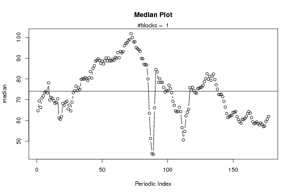
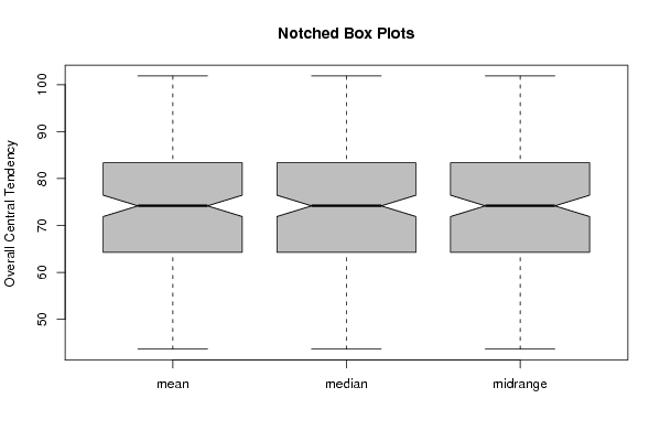
| Title produced by software | Mean Plot | ||||||||||||||||||||
| Date of computation | Thu, 25 Nov 2010 09:35:53 +0000 | ||||||||||||||||||||
| Cite this page as follows | Statistical Computations at FreeStatistics.org, Office for Research Development and Education, URL https://freestatistics.org/blog/index.php?v=date/2010/Nov/25/t12906776478xxrp83f83g1bdv.htm/, Retrieved Thu, 18 Apr 2024 12:50:34 +0000 | ||||||||||||||||||||
| Statistical Computations at FreeStatistics.org, Office for Research Development and Education, URL https://freestatistics.org/blog/index.php?pk=100665, Retrieved Thu, 18 Apr 2024 12:50:34 +0000 | |||||||||||||||||||||
| QR Codes: | |||||||||||||||||||||
|
| |||||||||||||||||||||
| Original text written by user: | |||||||||||||||||||||
| IsPrivate? | No (this computation is public) | ||||||||||||||||||||
| User-defined keywords | |||||||||||||||||||||
| Estimated Impact | 129 | ||||||||||||||||||||
Tree of Dependent Computations | |||||||||||||||||||||
| Family? (F = Feedback message, R = changed R code, M = changed R Module, P = changed Parameters, D = changed Data) | |||||||||||||||||||||
| - [Mean Plot] [] [2010-11-24 15:28:23] [43e84bd88d5f94b739fa54f225367516] - [Mean Plot] [] [2010-11-25 09:35:53] [19046f4a6967f3fb6f5f17d42e7d38f2] [Current] | |||||||||||||||||||||
| Feedback Forum | |||||||||||||||||||||
Post a new message | |||||||||||||||||||||
Dataset | |||||||||||||||||||||
| Dataseries X: | |||||||||||||||||||||
67.643 69.371 66.294 70.768 71.774 73.388 74.040 73.238 78.121 69.825 71.099 70.676 69.515 68.246 68.594 70.405 61.223 60.542 61.952 68.173 67.240 68.739 69.234 65.570 67.408 64.630 68.848 73.370 74.292 76.525 74.368 75.674 74.868 79.824 80.022 79.942 80.622 80.079 79.212 80.626 83.551 80.407 85.053 86.399 88.536 89.008 89.652 88.904 87.472 88.631 87.221 88.759 90.127 88.709 90.030 88.697 88.762 89.475 88.936 90.411 90.004 92.725 90.252 93.226 92.575 93.125 95.987 97.175 97.321 98.577 99.026 101.851 99.958 97.875 97.927 95.149 94.551 93.999 93.297 89.901 89.742 87.096 86.863 86.718 80.020 63.483 51.289 44.071 43.654 66.115 84.518 83.395 78.307 80.049 78.346 78.317 75.918 73.739 74.530 74.179 76.974 75.408 73.336 69.210 67.286 64.606 64.159 64.423 66.411 64.270 56.521 50.599 54.751 62.227 63.932 65.391 75.744 74.590 76.035 74.427 73.354 73.081 75.309 75.463 75.910 76.151 76.882 78.632 80.137 82.490 79.896 81.303 79.344 81.355 82.328 79.669 77.249 75.101 72.520 72.438 72.653 71.429 69.189 66.451 63.354 61.379 61.880 62.274 62.429 63.905 63.917 64.295 61.930 60.440 59.353 58.695 60.569 60.386 60.938 61.795 63.304 64.270 63.492 61.333 59.341 58.412 58.725 59.277 58.562 57.858 58.790 58.243 57.044 57.339 59.429 60.575 61.950 61.712 | |||||||||||||||||||||
Tables (Output of Computation) | |||||||||||||||||||||
| |||||||||||||||||||||
Figures (Output of Computation) | |||||||||||||||||||||
Input Parameters & R Code | |||||||||||||||||||||
| Parameters (Session): | |||||||||||||||||||||
| par1 = 177 ; | |||||||||||||||||||||
| Parameters (R input): | |||||||||||||||||||||
| par1 = 177 ; par2 = ; par3 = ; par4 = ; par5 = ; par6 = ; par7 = ; par8 = ; par9 = ; par10 = ; par11 = ; par12 = ; par13 = ; par14 = ; par15 = ; par16 = ; par17 = ; par18 = ; par19 = ; par20 = ; | |||||||||||||||||||||
| R code (references can be found in the software module): | |||||||||||||||||||||
par1 <- as.numeric(par1) | |||||||||||||||||||||