Free Statistics
of Irreproducible Research!
Description of Statistical Computation | |||||||||||||||||||||||||||||||||||||||||||||||||||||||||||||
|---|---|---|---|---|---|---|---|---|---|---|---|---|---|---|---|---|---|---|---|---|---|---|---|---|---|---|---|---|---|---|---|---|---|---|---|---|---|---|---|---|---|---|---|---|---|---|---|---|---|---|---|---|---|---|---|---|---|---|---|---|---|
| Author's title | |||||||||||||||||||||||||||||||||||||||||||||||||||||||||||||
| Author | *The author of this computation has been verified* | ||||||||||||||||||||||||||||||||||||||||||||||||||||||||||||
| R Software Module | rwasp_linear_regression.wasp | ||||||||||||||||||||||||||||||||||||||||||||||||||||||||||||
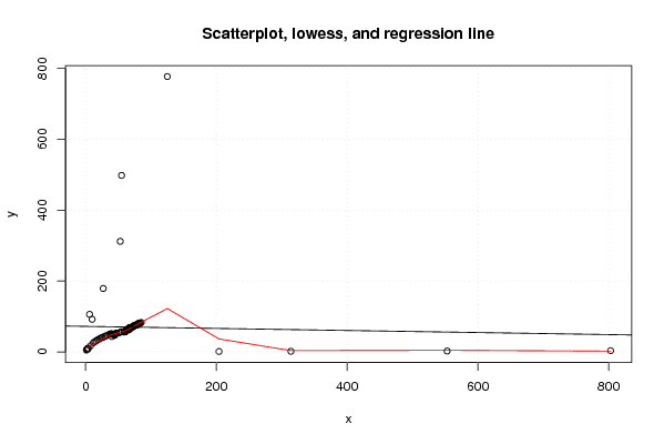
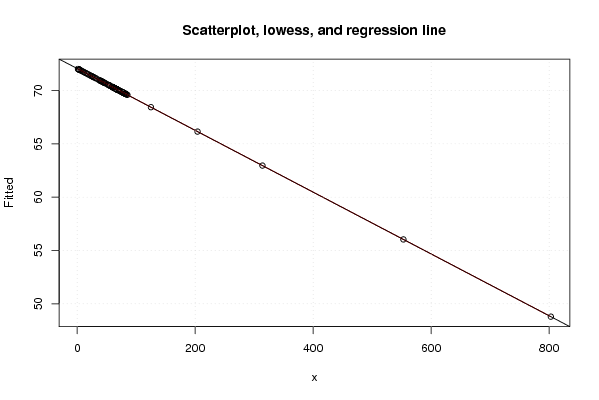
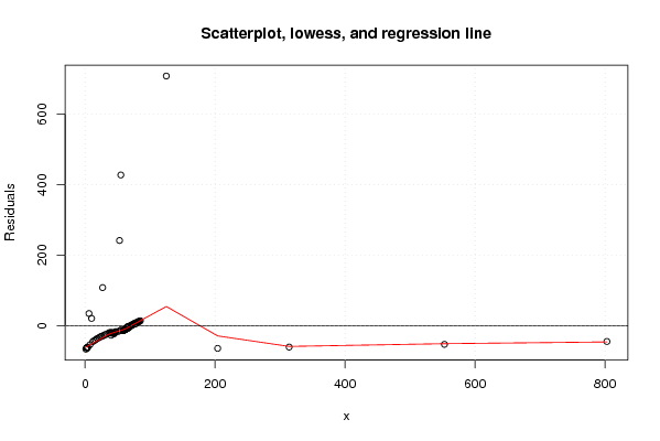
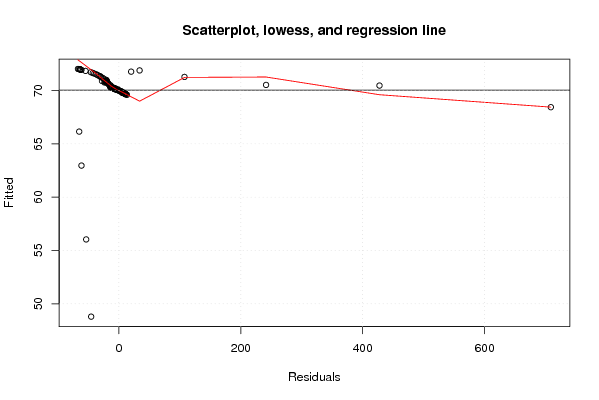
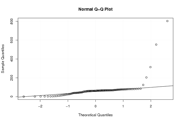
| Title produced by software | Linear Regression Graphical Model Validation | ||||||||||||||||||||||||||||||||||||||||||||||||||||||||||||
| Date of computation | Thu, 25 Nov 2010 11:12:40 +0000 | ||||||||||||||||||||||||||||||||||||||||||||||||||||||||||||
| Cite this page as follows | Statistical Computations at FreeStatistics.org, Office for Research Development and Education, URL https://freestatistics.org/blog/index.php?v=date/2010/Nov/25/t1290683544ez8rm0w16c5q1j1.htm/, Retrieved Tue, 16 Apr 2024 10:42:25 +0000 | ||||||||||||||||||||||||||||||||||||||||||||||||||||||||||||
| Statistical Computations at FreeStatistics.org, Office for Research Development and Education, URL https://freestatistics.org/blog/index.php?pk=100790, Retrieved Tue, 16 Apr 2024 10:42:25 +0000 | |||||||||||||||||||||||||||||||||||||||||||||||||||||||||||||
| QR Codes: | |||||||||||||||||||||||||||||||||||||||||||||||||||||||||||||
|
| |||||||||||||||||||||||||||||||||||||||||||||||||||||||||||||
| Original text written by user: | |||||||||||||||||||||||||||||||||||||||||||||||||||||||||||||
| IsPrivate? | No (this computation is public) | ||||||||||||||||||||||||||||||||||||||||||||||||||||||||||||
| User-defined keywords | |||||||||||||||||||||||||||||||||||||||||||||||||||||||||||||
| Estimated Impact | 125 | ||||||||||||||||||||||||||||||||||||||||||||||||||||||||||||
Tree of Dependent Computations | |||||||||||||||||||||||||||||||||||||||||||||||||||||||||||||
| Family? (F = Feedback message, R = changed R code, M = changed R Module, P = changed Parameters, D = changed Data) | |||||||||||||||||||||||||||||||||||||||||||||||||||||||||||||
| - [Linear Regression Graphical Model Validation] [Colombia Coffee -...] [2008-02-26 10:22:06] [74be16979710d4c4e7c6647856088456] - M D [Linear Regression Graphical Model Validation] [] [2010-11-25 11:12:40] [288f03f47c5783dcaccb816dacc66894] [Current] - D [Linear Regression Graphical Model Validation] [] [2010-11-26 14:52:17] [b85d3508e7cb050fe9be80ea93d51170] - D [Linear Regression Graphical Model Validation] [] [2010-11-26 14:52:17] [b85d3508e7cb050fe9be80ea93d51170] - P [Linear Regression Graphical Model Validation] [] [2010-12-13 20:07:13] [e71d94d32f847f62b540eebe6fadd003] - P [Linear Regression Graphical Model Validation] [] [2010-12-13 20:07:13] [43e84bd88d5f94b739fa54f225367516] - P [Linear Regression Graphical Model Validation] [] [2010-12-13 20:07:13] [43e84bd88d5f94b739fa54f225367516] | |||||||||||||||||||||||||||||||||||||||||||||||||||||||||||||
| Feedback Forum | |||||||||||||||||||||||||||||||||||||||||||||||||||||||||||||
Post a new message | |||||||||||||||||||||||||||||||||||||||||||||||||||||||||||||
Dataset | |||||||||||||||||||||||||||||||||||||||||||||||||||||||||||||
| Dataseries X: | |||||||||||||||||||||||||||||||||||||||||||||||||||||||||||||
61.712 62.084 61.406 60.724 58.904 58.722 59.704 60.674 59.813 60.568 61.401 61.427 61.080 61.999 63.888 66.284 67.309 66.685 65.404 65.045 63.867 64.156 62.224 63.193 64.256 66.153 68.072 68.245 68.741 67.795 67.315 67.245 66.448 69.112 71.787 74.366 76.337 77.618 77.090 76.925 78.384 80.462 82.765 85.033 83.608 81.813 81.467 80.708 80.631 79.133 77.396 75.491 74.267 72.882 71.286 70.737 67.425 67.530 67.157 67.215 66.268 66.053 54.905 54.459 51.159 44.725 40.184 44.094 46.904 47.141 45.052 42.758 41.388 41.154 40.019 39.928 38.598 36.584 32.566 30.140 27.713 25.380 23.823 21.376 18.696 16.304 14.203 11.807 7.551 4.215 3.346 3.010 2.849 2.485 1.744 1.221 803 553 314 204 125 55 53 27 10 6 | |||||||||||||||||||||||||||||||||||||||||||||||||||||||||||||
| Dataseries Y: | |||||||||||||||||||||||||||||||||||||||||||||||||||||||||||||
58.951 59.634 58.389 57.702 56.593 55.998 57.363 58.022 57.598 57.842 58.875 59.103 58.484 58.636 61.342 63.470 64.281 63.721 62.657 62.549 61.882 62.325 61.907 63.136 63.982 65.800 67.596 68.654 67.548 67.398 66.999 66.284 65.561 67.694 69.976 72.908 75.128 75.522 75.242 75.179 75.572 78.340 80.107 82.972 81.638 80.018 80.631 79.211 79.999 77.789 76.205 75.352 74.393 72.771 70.682 69.991 67.525 67.779 66.864 67.971 67.071 66.980 57.144 56.648 53.706 47.108 43.292 48.489 52.642 53.249 50.722 49.805 49.303 49.985 49.512 51.282 50.734 50.365 46.191 44.617 42.012 41.027 39.478 36.824 34.761 31.295 28.951 25.872 17.297 10.739 9.087 8.658 8.731 8.358 6.518 5.021 3.440 2.523 1.725 1.210 777 498 312 179 92 106 | |||||||||||||||||||||||||||||||||||||||||||||||||||||||||||||
Tables (Output of Computation) | |||||||||||||||||||||||||||||||||||||||||||||||||||||||||||||
| |||||||||||||||||||||||||||||||||||||||||||||||||||||||||||||
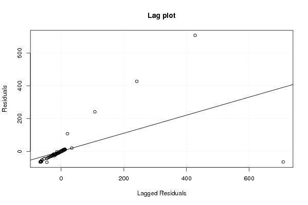
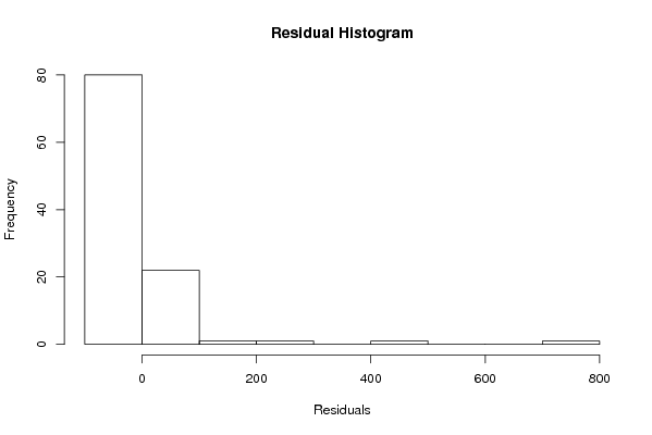
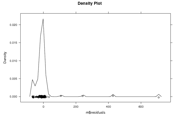
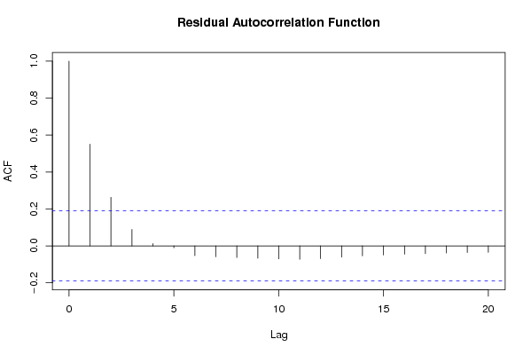
Figures (Output of Computation) | |||||||||||||||||||||||||||||||||||||||||||||||||||||||||||||
Input Parameters & R Code | |||||||||||||||||||||||||||||||||||||||||||||||||||||||||||||
| Parameters (Session): | |||||||||||||||||||||||||||||||||||||||||||||||||||||||||||||
| par1 = 0 ; | |||||||||||||||||||||||||||||||||||||||||||||||||||||||||||||
| Parameters (R input): | |||||||||||||||||||||||||||||||||||||||||||||||||||||||||||||
| par1 = 0 ; | |||||||||||||||||||||||||||||||||||||||||||||||||||||||||||||
| R code (references can be found in the software module): | |||||||||||||||||||||||||||||||||||||||||||||||||||||||||||||
par1 <- as.numeric(par1) | |||||||||||||||||||||||||||||||||||||||||||||||||||||||||||||