Free Statistics
of Irreproducible Research!
Description of Statistical Computation | |||||||||||||||||||||||||||||||||||||||||||||||||||||||||||||
|---|---|---|---|---|---|---|---|---|---|---|---|---|---|---|---|---|---|---|---|---|---|---|---|---|---|---|---|---|---|---|---|---|---|---|---|---|---|---|---|---|---|---|---|---|---|---|---|---|---|---|---|---|---|---|---|---|---|---|---|---|---|
| Author's title | |||||||||||||||||||||||||||||||||||||||||||||||||||||||||||||
| Author | *The author of this computation has been verified* | ||||||||||||||||||||||||||||||||||||||||||||||||||||||||||||
| R Software Module | rwasp_linear_regression.wasp | ||||||||||||||||||||||||||||||||||||||||||||||||||||||||||||
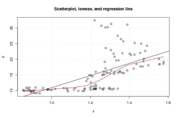
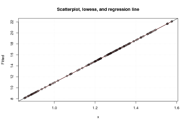
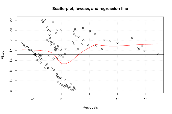
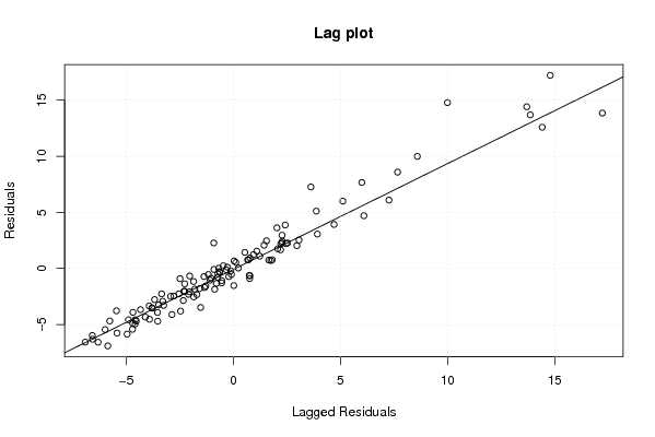
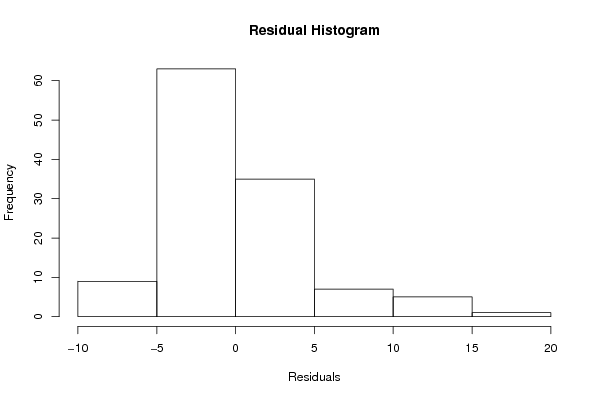
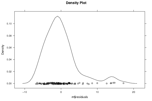
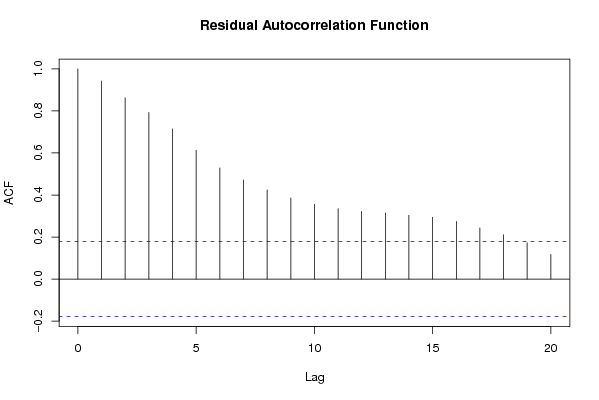
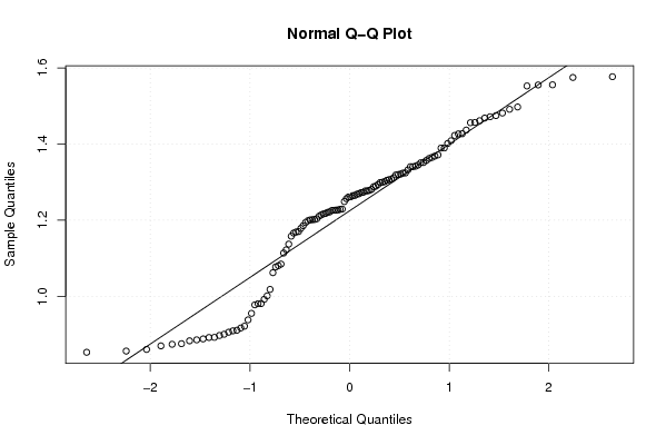
| Title produced by software | Linear Regression Graphical Model Validation | ||||||||||||||||||||||||||||||||||||||||||||||||||||||||||||
| Date of computation | Thu, 25 Nov 2010 18:35:56 +0000 | ||||||||||||||||||||||||||||||||||||||||||||||||||||||||||||
| Cite this page as follows | Statistical Computations at FreeStatistics.org, Office for Research Development and Education, URL https://freestatistics.org/blog/index.php?v=date/2010/Nov/25/t12907100901scg9u5g93ei0hg.htm/, Retrieved Tue, 23 Apr 2024 23:09:19 +0000 | ||||||||||||||||||||||||||||||||||||||||||||||||||||||||||||
| Statistical Computations at FreeStatistics.org, Office for Research Development and Education, URL https://freestatistics.org/blog/index.php?pk=101334, Retrieved Tue, 23 Apr 2024 23:09:19 +0000 | |||||||||||||||||||||||||||||||||||||||||||||||||||||||||||||
| QR Codes: | |||||||||||||||||||||||||||||||||||||||||||||||||||||||||||||
|
| |||||||||||||||||||||||||||||||||||||||||||||||||||||||||||||
| Original text written by user: | |||||||||||||||||||||||||||||||||||||||||||||||||||||||||||||
| IsPrivate? | No (this computation is public) | ||||||||||||||||||||||||||||||||||||||||||||||||||||||||||||
| User-defined keywords | |||||||||||||||||||||||||||||||||||||||||||||||||||||||||||||
| Estimated Impact | 120 | ||||||||||||||||||||||||||||||||||||||||||||||||||||||||||||
Tree of Dependent Computations | |||||||||||||||||||||||||||||||||||||||||||||||||||||||||||||
| Family? (F = Feedback message, R = changed R code, M = changed R Module, P = changed Parameters, D = changed Data) | |||||||||||||||||||||||||||||||||||||||||||||||||||||||||||||
| - [Linear Regression Graphical Model Validation] [Colombia Coffee -...] [2008-02-26 10:22:06] [74be16979710d4c4e7c6647856088456] - M D [Linear Regression Graphical Model Validation] [] [2010-11-25 09:23:05] [4dfa50539945b119a90a7606969443b9] - D [Linear Regression Graphical Model Validation] [] [2010-11-25 18:35:56] [cf84dc108eae081aed36d3d050e63ee7] [Current] | |||||||||||||||||||||||||||||||||||||||||||||||||||||||||||||
| Feedback Forum | |||||||||||||||||||||||||||||||||||||||||||||||||||||||||||||
Post a new message | |||||||||||||||||||||||||||||||||||||||||||||||||||||||||||||
Dataset | |||||||||||||||||||||||||||||||||||||||||||||||||||||||||||||
| Dataseries X: | |||||||||||||||||||||||||||||||||||||||||||||||||||||||||||||
1,3898 1,3067 1,2894 1,277 1,2208 1,2565 1,3406 1,3569 1,3686 1,4272 1,4614 1,4914 1,4816 1,4562 1,4268 1,4088 1,4016 1,365 1,319 1,305 1,2785 1,3239 1,3449 1,2732 1,3322 1,4369 1,4975 1,577 1,5553 1,5557 1,575 1,5527 1,4748 1,4718 1,457 1,4684 1,4227 1,3896 1,3622 1,3716 1,3419 1,3511 1,3516 1,3242 1,3074 1,2999 1,3213 1,2881 1,2611 1,2727 1,2811 1,2684 1,265 1,277 1,2271 1,202 1,1938 1,2103 1,1856 1,1786 1,2015 1,2256 1,2292 1,2037 1,2165 1,2694 1,2938 1,3201 1,3014 1,3119 1,3408 1,2991 1,249 1,2218 1,2176 1,2266 1,2138 1,2007 1,1985 1,2262 1,2646 1,2613 1,2286 1,1702 1,1692 1,1222 1,1139 1,1372 1,1663 1,1582 1,0848 1,0807 1,0773 1,0622 1,0183 1,0014 0,9811 0,9808 0,9778 0,9922 0,9554 0,917 0,8858 0,8758 0,87 0,8833 0,8924 0,8883 0,9059 0,9111 0,9005 0,8607 0,8532 0,8742 0,892 0,9095 0,9217 0,9383 0,8973 0,8564 | |||||||||||||||||||||||||||||||||||||||||||||||||||||||||||||
| Dataseries Y: | |||||||||||||||||||||||||||||||||||||||||||||||||||||||||||||
31,077 31,293 30,236 30,160 32,436 30,695 27,525 26,434 25,739 25,204 24,977 24,320 22,680 22,052 21,467 21,383 21,777 21,928 21,814 22,937 23,595 20,830 19,650 19,195 19,644 18,483 18,079 19,178 18,391 18,441 18,584 20,108 20,148 19,394 17,745 17,696 17,032 16,438 15,683 15,594 15,713 15,937 16,171 15,928 16,348 15,579 15,305 15,648 14,954 15,137 15,839 16,050 15,168 17,064 16,005 14,886 14,931 14,544 13,812 13,031 12,574 11,964 11,451 11,346 11,353 10,702 10,646 10,556 10,463 10,407 10,625 10,872 10,805 10,653 10,574 10,431 10,383 10,296 10,872 10,635 10,297 10,570 10,662 10,709 10,413 10,846 10,371 9,924 9,828 9,897 9,721 10,171 10,738 10,812 10,511 10,244 10,368 10,457 10,186 10,166 10,827 10,997 10,940 10,756 10,893 10,236 9,960 10,018 10,063 10,002 9,728 10,002 10,177 9,948 9,394 9,308 9,155 9,103 9,732 9,984 | |||||||||||||||||||||||||||||||||||||||||||||||||||||||||||||
Tables (Output of Computation) | |||||||||||||||||||||||||||||||||||||||||||||||||||||||||||||
| |||||||||||||||||||||||||||||||||||||||||||||||||||||||||||||
Figures (Output of Computation) | |||||||||||||||||||||||||||||||||||||||||||||||||||||||||||||
Input Parameters & R Code | |||||||||||||||||||||||||||||||||||||||||||||||||||||||||||||
| Parameters (Session): | |||||||||||||||||||||||||||||||||||||||||||||||||||||||||||||
| par1 = 0 ; | |||||||||||||||||||||||||||||||||||||||||||||||||||||||||||||
| Parameters (R input): | |||||||||||||||||||||||||||||||||||||||||||||||||||||||||||||
| par1 = 0 ; | |||||||||||||||||||||||||||||||||||||||||||||||||||||||||||||
| R code (references can be found in the software module): | |||||||||||||||||||||||||||||||||||||||||||||||||||||||||||||
par1 <- as.numeric(par1) | |||||||||||||||||||||||||||||||||||||||||||||||||||||||||||||