Repository of Reproducible Computations

Free Statistics

of Irreproducible Research!

Author's title

Author

*The author of this computation has been verified*

R Software Module

rwasp_autocorrelation.wasp

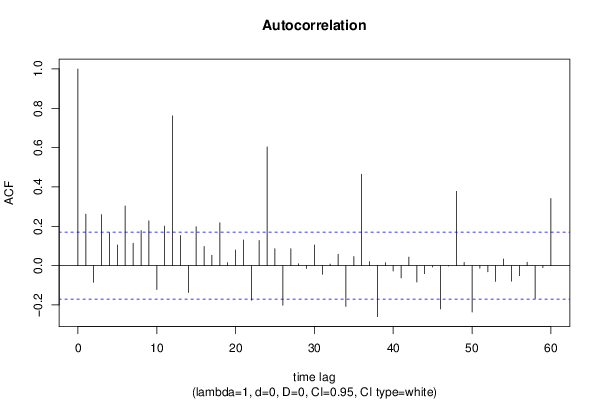
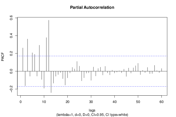
Title produced by software

(Partial) Autocorrelation Function

Date of computation

Sat, 10 Nov 2012 11:56:48 -0500

Cite this page as follows

Statistical Computations at FreeStatistics.org, Office for Research Development and Education, URL https://freestatistics.org/blog/index.php?v=date/2012/Nov/10/t1352566697pdgqijicfdtgi1a.htm/, Retrieved Fri, 19 Apr 2024 21:28:44 +0000

Statistical Computations at FreeStatistics.org, Office for Research Development and Education, URL https://freestatistics.org/blog/index.php?pk=187389, Retrieved Fri, 19 Apr 2024 21:28:44 +0000

QR Codes:

Paste this QR Code to cite your computation.

Original text written by user:

IsPrivate?

No (this computation is public)

User-defined keywords

Estimated Impact

122

Family? (F = Feedback message, R = changed R code, M = changed R Module, P = changed Parameters, D = changed Data)

F     [Univariate Data Series] [HPC Retail Sales] [2008-03-02 15:42:48] [74be16979710d4c4e7c6647856088456]
- RMPD    [(Partial) Autocorrelation Function] [Autocorrelatiefun...] [2012-11-10 16:56:48] [7338cd26db379c04f0557b08db763c32] [Current]
- R P       [(Partial) Autocorrelation Function] [] [2012-11-24 00:03:24] [74be16979710d4c4e7c6647856088456] 
-   P         [(Partial) Autocorrelation Function] [Langetermijntrend...] [2012-11-24 09:07:33] [74be16979710d4c4e7c6647856088456] 
-   P           [(Partial) Autocorrelation Function] [Seizoenale differ...] [2012-11-24 09:21:40] [74be16979710d4c4e7c6647856088456] 
-  M              [(Partial) Autocorrelation Function] [] [2012-12-20 19:29:27] [74be16979710d4c4e7c6647856088456] 
- RMP           [Spectral Analysis] [Cumm.Periodogram_...] [2012-11-24 09:46:23] [391561951b5d7f721cfaa4f5575ab127] 
- RM              [Spectral Analysis] [] [2012-12-20 19:31:14] [74be16979710d4c4e7c6647856088456] 
- RMP           [Spectral Analysis] [Differentiatie_Cu...] [2012-11-24 09:54:01] [391561951b5d7f721cfaa4f5575ab127] 
- RM              [Spectral Analysis] [] [2012-12-20 19:32:43] [74be16979710d4c4e7c6647856088456] 
- RMP           [Spectral Analysis] [Stationaritair di...] [2012-11-24 10:11:58] [391561951b5d7f721cfaa4f5575ab127] 
- RM              [Spectral Analysis] [] [2012-12-20 19:34:10] [74be16979710d4c4e7c6647856088456] 
- RMP           [Variance Reduction Matrix] [Variance Reductio...] [2012-11-24 10:29:02] [391561951b5d7f721cfaa4f5575ab127] 
- RM              [Variance Reduction Matrix] [] [2012-12-20 19:35:43] [74be16979710d4c4e7c6647856088456] 
- RMP           [Variance Reduction Matrix] [] [2012-11-24 10:40:27] [391561951b5d7f721cfaa4f5575ab127] 
- RMP           [Standard Deviation-Mean Plot] [] [2012-11-24 10:58:52] [391561951b5d7f721cfaa4f5575ab127] 
- RM              [Standard Deviation-Mean Plot] [] [2012-12-20 19:40:31] [74be16979710d4c4e7c6647856088456] 
-               [(Partial) Autocorrelation Function] [] [2012-11-26 20:30:00] [391561951b5d7f721cfaa4f5575ab127] 
-  M            [(Partial) Autocorrelation Function] [] [2012-12-20 19:20:26] [74be16979710d4c4e7c6647856088456] 
-  M          [(Partial) Autocorrelation Function] [] [2012-12-20 17:40:37] [74be16979710d4c4e7c6647856088456] 

Feedback Forum

Post a new message

Dataseries X:

Download CSV

Histogram

Boxplots

Summary of computational transaction
Raw Input	view raw input (R code)
Raw Output	view raw output of R engine
Computing time	3 seconds
R Server	'George Udny Yule' @ yule.wessa.net

\begin{tabular}{lllllllll}
\hline
Summary of computational transaction \tabularnewline
Raw Input & view raw input (R code)  \tabularnewline
Raw Output & view raw output of R engine  \tabularnewline
Computing time & 3 seconds \tabularnewline
R Server & 'George Udny Yule' @ yule.wessa.net \tabularnewline
\hline
\end{tabular}
%Source: https://freestatistics.org/blog/index.php?pk=187389&T=0

[TABLE]
[ROW][C]Summary of computational transaction[/C][/ROW]
[ROW][C]Raw Input[/C][C]view raw input (R code) [/C][/ROW]
[ROW][C]Raw Output[/C][C]view raw output of R engine [/C][/ROW]
[ROW][C]Computing time[/C][C]3 seconds[/C][/ROW]
[ROW][C]R Server[/C][C]'George Udny Yule' @ yule.wessa.net[/C][/ROW]
[/TABLE]
Source: https://freestatistics.org/blog/index.php?pk=187389&T=0

Globally Unique Identifier (entire table): ba.freestatistics.org/blog/index.php?pk=187389&T=0

As an alternative you can also use a QR Code:

The GUIDs for individual cells are displayed in the table below:

Summary of computational transaction
Raw Input	view raw input (R code)
Raw Output	view raw output of R engine
Computing time	3 seconds
R Server	'George Udny Yule' @ yule.wessa.net

Autocorrelation Function
Time lag k	ACF(k)	T-STAT	P-value
1	0.26182	3.0081	0.001575
2	-0.084377	-0.9694	0.167056
3	0.259481	2.9812	0.00171
4	0.167974	1.9299	0.027884
5	0.105202	1.2087	0.114473
6	0.30295	3.4806	0.000339
7	0.113661	1.3059	0.096935
8	0.178119	2.0464	0.02135
9	0.22773	2.6164	0.004961
10	-0.121433	-1.3952	0.082655
11	0.201112	2.3106	0.011203
12	0.761335	8.7471	0
13	0.153289	1.7612	0.040264
14	-0.136579	-1.5692	0.059501
15	0.197495	2.269	0.012444
16	0.097637	1.1218	0.131999
17	0.052279	0.6006	0.274555
18	0.218558	2.511	0.006622
19	0.015508	0.1782	0.429431
20	0.079433	0.9126	0.181553
21	0.130346	1.4976	0.068318
22	-0.175396	-2.0152	0.02296
23	0.128256	1.4736	0.071492
24	0.603337	6.9318	0
25	0.086067	0.9888	0.162277
26	-0.200928	-2.3085	0.011263
27	0.08611	0.9893	0.162155
28	0.009746	0.112	0.455509
29	-0.014056	-0.1615	0.435978
30	0.105023	1.2066	0.114867
31	-0.043763	-0.5028	0.307974
32	0.007843	0.0901	0.46417
33	0.057884	0.665	0.253594
34	-0.207092	-2.3793	0.009389
35	0.045818	0.5264	0.299744
36	0.464353	5.335	0
37	0.020613	0.2368	0.40658
38	-0.25927	-2.9788	0.001723
39	0.014968	0.172	0.431861
40	-0.027104	-0.3114	0.377994
41	-0.062299	-0.7158	0.237701
42	0.043364	0.4982	0.309579
43	-0.082983	-0.9534	0.171065
44	-0.040542	-0.4658	0.321066
45	-0.006926	-0.0796	0.468349
46	-0.21969	-2.524	0.006393
47	-0.001667	-0.0192	0.492372
48	0.377789	4.3405	1.4e-05
49	0.015911	0.1828	0.427618
50	-0.235395	-2.7045	0.003871
51	-0.013069	-0.1501	0.440439
52	-0.03099	-0.356	0.361187
53	-0.079942	-0.9185	0.180025
54	0.034017	0.3908	0.34828
55	-0.078724	-0.9045	0.183698
56	-0.051097	-0.5871	0.279083
57	0.016943	0.1947	0.422978
58	-0.167016	-1.9189	0.02858
59	-0.010208	-0.1173	0.453409
60	0.341065	3.9185	7.1e-05

\begin{tabular}{lllllllll}
\hline
Autocorrelation Function \tabularnewline
Time lag k & ACF(k) & T-STAT & P-value \tabularnewline
1 & 0.26182 & 3.0081 & 0.001575 \tabularnewline
2 & -0.084377 & -0.9694 & 0.167056 \tabularnewline
3 & 0.259481 & 2.9812 & 0.00171 \tabularnewline
4 & 0.167974 & 1.9299 & 0.027884 \tabularnewline
5 & 0.105202 & 1.2087 & 0.114473 \tabularnewline
6 & 0.30295 & 3.4806 & 0.000339 \tabularnewline
7 & 0.113661 & 1.3059 & 0.096935 \tabularnewline
8 & 0.178119 & 2.0464 & 0.02135 \tabularnewline
9 & 0.22773 & 2.6164 & 0.004961 \tabularnewline
10 & -0.121433 & -1.3952 & 0.082655 \tabularnewline
11 & 0.201112 & 2.3106 & 0.011203 \tabularnewline
12 & 0.761335 & 8.7471 & 0 \tabularnewline
13 & 0.153289 & 1.7612 & 0.040264 \tabularnewline
14 & -0.136579 & -1.5692 & 0.059501 \tabularnewline
15 & 0.197495 & 2.269 & 0.012444 \tabularnewline
16 & 0.097637 & 1.1218 & 0.131999 \tabularnewline
17 & 0.052279 & 0.6006 & 0.274555 \tabularnewline
18 & 0.218558 & 2.511 & 0.006622 \tabularnewline
19 & 0.015508 & 0.1782 & 0.429431 \tabularnewline
20 & 0.079433 & 0.9126 & 0.181553 \tabularnewline
21 & 0.130346 & 1.4976 & 0.068318 \tabularnewline
22 & -0.175396 & -2.0152 & 0.02296 \tabularnewline
23 & 0.128256 & 1.4736 & 0.071492 \tabularnewline
24 & 0.603337 & 6.9318 & 0 \tabularnewline
25 & 0.086067 & 0.9888 & 0.162277 \tabularnewline
26 & -0.200928 & -2.3085 & 0.011263 \tabularnewline
27 & 0.08611 & 0.9893 & 0.162155 \tabularnewline
28 & 0.009746 & 0.112 & 0.455509 \tabularnewline
29 & -0.014056 & -0.1615 & 0.435978 \tabularnewline
30 & 0.105023 & 1.2066 & 0.114867 \tabularnewline
31 & -0.043763 & -0.5028 & 0.307974 \tabularnewline
32 & 0.007843 & 0.0901 & 0.46417 \tabularnewline
33 & 0.057884 & 0.665 & 0.253594 \tabularnewline
34 & -0.207092 & -2.3793 & 0.009389 \tabularnewline
35 & 0.045818 & 0.5264 & 0.299744 \tabularnewline
36 & 0.464353 & 5.335 & 0 \tabularnewline
37 & 0.020613 & 0.2368 & 0.40658 \tabularnewline
38 & -0.25927 & -2.9788 & 0.001723 \tabularnewline
39 & 0.014968 & 0.172 & 0.431861 \tabularnewline
40 & -0.027104 & -0.3114 & 0.377994 \tabularnewline
41 & -0.062299 & -0.7158 & 0.237701 \tabularnewline
42 & 0.043364 & 0.4982 & 0.309579 \tabularnewline
43 & -0.082983 & -0.9534 & 0.171065 \tabularnewline
44 & -0.040542 & -0.4658 & 0.321066 \tabularnewline
45 & -0.006926 & -0.0796 & 0.468349 \tabularnewline
46 & -0.21969 & -2.524 & 0.006393 \tabularnewline
47 & -0.001667 & -0.0192 & 0.492372 \tabularnewline
48 & 0.377789 & 4.3405 & 1.4e-05 \tabularnewline
49 & 0.015911 & 0.1828 & 0.427618 \tabularnewline
50 & -0.235395 & -2.7045 & 0.003871 \tabularnewline
51 & -0.013069 & -0.1501 & 0.440439 \tabularnewline
52 & -0.03099 & -0.356 & 0.361187 \tabularnewline
53 & -0.079942 & -0.9185 & 0.180025 \tabularnewline
54 & 0.034017 & 0.3908 & 0.34828 \tabularnewline
55 & -0.078724 & -0.9045 & 0.183698 \tabularnewline
56 & -0.051097 & -0.5871 & 0.279083 \tabularnewline
57 & 0.016943 & 0.1947 & 0.422978 \tabularnewline
58 & -0.167016 & -1.9189 & 0.02858 \tabularnewline
59 & -0.010208 & -0.1173 & 0.453409 \tabularnewline
60 & 0.341065 & 3.9185 & 7.1e-05 \tabularnewline
\hline
\end{tabular}
%Source: https://freestatistics.org/blog/index.php?pk=187389&T=1

[TABLE]
[ROW][C]Autocorrelation Function[/C][/ROW]
[ROW][C]Time lag k[/C][C]ACF(k)[/C][C]T-STAT[/C][C]P-value[/C][/ROW]
[ROW][C]1[/C][C]0.26182[/C][C]3.0081[/C][C]0.001575[/C][/ROW]
[ROW][C]2[/C][C]-0.084377[/C][C]-0.9694[/C][C]0.167056[/C][/ROW]
[ROW][C]3[/C][C]0.259481[/C][C]2.9812[/C][C]0.00171[/C][/ROW]
[ROW][C]4[/C][C]0.167974[/C][C]1.9299[/C][C]0.027884[/C][/ROW]
[ROW][C]5[/C][C]0.105202[/C][C]1.2087[/C][C]0.114473[/C][/ROW]
[ROW][C]6[/C][C]0.30295[/C][C]3.4806[/C][C]0.000339[/C][/ROW]
[ROW][C]7[/C][C]0.113661[/C][C]1.3059[/C][C]0.096935[/C][/ROW]
[ROW][C]8[/C][C]0.178119[/C][C]2.0464[/C][C]0.02135[/C][/ROW]
[ROW][C]9[/C][C]0.22773[/C][C]2.6164[/C][C]0.004961[/C][/ROW]
[ROW][C]10[/C][C]-0.121433[/C][C]-1.3952[/C][C]0.082655[/C][/ROW]
[ROW][C]11[/C][C]0.201112[/C][C]2.3106[/C][C]0.011203[/C][/ROW]
[ROW][C]12[/C][C]0.761335[/C][C]8.7471[/C][C]0[/C][/ROW]
[ROW][C]13[/C][C]0.153289[/C][C]1.7612[/C][C]0.040264[/C][/ROW]
[ROW][C]14[/C][C]-0.136579[/C][C]-1.5692[/C][C]0.059501[/C][/ROW]
[ROW][C]15[/C][C]0.197495[/C][C]2.269[/C][C]0.012444[/C][/ROW]
[ROW][C]16[/C][C]0.097637[/C][C]1.1218[/C][C]0.131999[/C][/ROW]
[ROW][C]17[/C][C]0.052279[/C][C]0.6006[/C][C]0.274555[/C][/ROW]
[ROW][C]18[/C][C]0.218558[/C][C]2.511[/C][C]0.006622[/C][/ROW]
[ROW][C]19[/C][C]0.015508[/C][C]0.1782[/C][C]0.429431[/C][/ROW]
[ROW][C]20[/C][C]0.079433[/C][C]0.9126[/C][C]0.181553[/C][/ROW]
[ROW][C]21[/C][C]0.130346[/C][C]1.4976[/C][C]0.068318[/C][/ROW]
[ROW][C]22[/C][C]-0.175396[/C][C]-2.0152[/C][C]0.02296[/C][/ROW]
[ROW][C]23[/C][C]0.128256[/C][C]1.4736[/C][C]0.071492[/C][/ROW]
[ROW][C]24[/C][C]0.603337[/C][C]6.9318[/C][C]0[/C][/ROW]
[ROW][C]25[/C][C]0.086067[/C][C]0.9888[/C][C]0.162277[/C][/ROW]
[ROW][C]26[/C][C]-0.200928[/C][C]-2.3085[/C][C]0.011263[/C][/ROW]
[ROW][C]27[/C][C]0.08611[/C][C]0.9893[/C][C]0.162155[/C][/ROW]
[ROW][C]28[/C][C]0.009746[/C][C]0.112[/C][C]0.455509[/C][/ROW]
[ROW][C]29[/C][C]-0.014056[/C][C]-0.1615[/C][C]0.435978[/C][/ROW]
[ROW][C]30[/C][C]0.105023[/C][C]1.2066[/C][C]0.114867[/C][/ROW]
[ROW][C]31[/C][C]-0.043763[/C][C]-0.5028[/C][C]0.307974[/C][/ROW]
[ROW][C]32[/C][C]0.007843[/C][C]0.0901[/C][C]0.46417[/C][/ROW]
[ROW][C]33[/C][C]0.057884[/C][C]0.665[/C][C]0.253594[/C][/ROW]
[ROW][C]34[/C][C]-0.207092[/C][C]-2.3793[/C][C]0.009389[/C][/ROW]
[ROW][C]35[/C][C]0.045818[/C][C]0.5264[/C][C]0.299744[/C][/ROW]
[ROW][C]36[/C][C]0.464353[/C][C]5.335[/C][C]0[/C][/ROW]
[ROW][C]37[/C][C]0.020613[/C][C]0.2368[/C][C]0.40658[/C][/ROW]
[ROW][C]38[/C][C]-0.25927[/C][C]-2.9788[/C][C]0.001723[/C][/ROW]
[ROW][C]39[/C][C]0.014968[/C][C]0.172[/C][C]0.431861[/C][/ROW]
[ROW][C]40[/C][C]-0.027104[/C][C]-0.3114[/C][C]0.377994[/C][/ROW]
[ROW][C]41[/C][C]-0.062299[/C][C]-0.7158[/C][C]0.237701[/C][/ROW]
[ROW][C]42[/C][C]0.043364[/C][C]0.4982[/C][C]0.309579[/C][/ROW]
[ROW][C]43[/C][C]-0.082983[/C][C]-0.9534[/C][C]0.171065[/C][/ROW]
[ROW][C]44[/C][C]-0.040542[/C][C]-0.4658[/C][C]0.321066[/C][/ROW]
[ROW][C]45[/C][C]-0.006926[/C][C]-0.0796[/C][C]0.468349[/C][/ROW]
[ROW][C]46[/C][C]-0.21969[/C][C]-2.524[/C][C]0.006393[/C][/ROW]
[ROW][C]47[/C][C]-0.001667[/C][C]-0.0192[/C][C]0.492372[/C][/ROW]
[ROW][C]48[/C][C]0.377789[/C][C]4.3405[/C][C]1.4e-05[/C][/ROW]
[ROW][C]49[/C][C]0.015911[/C][C]0.1828[/C][C]0.427618[/C][/ROW]
[ROW][C]50[/C][C]-0.235395[/C][C]-2.7045[/C][C]0.003871[/C][/ROW]
[ROW][C]51[/C][C]-0.013069[/C][C]-0.1501[/C][C]0.440439[/C][/ROW]
[ROW][C]52[/C][C]-0.03099[/C][C]-0.356[/C][C]0.361187[/C][/ROW]
[ROW][C]53[/C][C]-0.079942[/C][C]-0.9185[/C][C]0.180025[/C][/ROW]
[ROW][C]54[/C][C]0.034017[/C][C]0.3908[/C][C]0.34828[/C][/ROW]
[ROW][C]55[/C][C]-0.078724[/C][C]-0.9045[/C][C]0.183698[/C][/ROW]
[ROW][C]56[/C][C]-0.051097[/C][C]-0.5871[/C][C]0.279083[/C][/ROW]
[ROW][C]57[/C][C]0.016943[/C][C]0.1947[/C][C]0.422978[/C][/ROW]
[ROW][C]58[/C][C]-0.167016[/C][C]-1.9189[/C][C]0.02858[/C][/ROW]
[ROW][C]59[/C][C]-0.010208[/C][C]-0.1173[/C][C]0.453409[/C][/ROW]
[ROW][C]60[/C][C]0.341065[/C][C]3.9185[/C][C]7.1e-05[/C][/ROW]
[/TABLE]
Source: https://freestatistics.org/blog/index.php?pk=187389&T=1

Globally Unique Identifier (entire table): ba.freestatistics.org/blog/index.php?pk=187389&T=1

As an alternative you can also use a QR Code:

The GUIDs for individual cells are displayed in the table below:

Autocorrelation Function
Time lag k	ACF(k)	T-STAT	P-value
1	0.26182	3.0081	0.001575
2	-0.084377	-0.9694	0.167056
3	0.259481	2.9812	0.00171
4	0.167974	1.9299	0.027884
5	0.105202	1.2087	0.114473
6	0.30295	3.4806	0.000339
7	0.113661	1.3059	0.096935
8	0.178119	2.0464	0.02135
9	0.22773	2.6164	0.004961
10	-0.121433	-1.3952	0.082655
11	0.201112	2.3106	0.011203
12	0.761335	8.7471	0
13	0.153289	1.7612	0.040264
14	-0.136579	-1.5692	0.059501
15	0.197495	2.269	0.012444
16	0.097637	1.1218	0.131999
17	0.052279	0.6006	0.274555
18	0.218558	2.511	0.006622
19	0.015508	0.1782	0.429431
20	0.079433	0.9126	0.181553
21	0.130346	1.4976	0.068318
22	-0.175396	-2.0152	0.02296
23	0.128256	1.4736	0.071492
24	0.603337	6.9318	0
25	0.086067	0.9888	0.162277
26	-0.200928	-2.3085	0.011263
27	0.08611	0.9893	0.162155
28	0.009746	0.112	0.455509
29	-0.014056	-0.1615	0.435978
30	0.105023	1.2066	0.114867
31	-0.043763	-0.5028	0.307974
32	0.007843	0.0901	0.46417
33	0.057884	0.665	0.253594
34	-0.207092	-2.3793	0.009389
35	0.045818	0.5264	0.299744
36	0.464353	5.335	0
37	0.020613	0.2368	0.40658
38	-0.25927	-2.9788	0.001723
39	0.014968	0.172	0.431861
40	-0.027104	-0.3114	0.377994
41	-0.062299	-0.7158	0.237701
42	0.043364	0.4982	0.309579
43	-0.082983	-0.9534	0.171065
44	-0.040542	-0.4658	0.321066
45	-0.006926	-0.0796	0.468349
46	-0.21969	-2.524	0.006393
47	-0.001667	-0.0192	0.492372
48	0.377789	4.3405	1.4e-05
49	0.015911	0.1828	0.427618
50	-0.235395	-2.7045	0.003871
51	-0.013069	-0.1501	0.440439
52	-0.03099	-0.356	0.361187
53	-0.079942	-0.9185	0.180025
54	0.034017	0.3908	0.34828
55	-0.078724	-0.9045	0.183698
56	-0.051097	-0.5871	0.279083
57	0.016943	0.1947	0.422978
58	-0.167016	-1.9189	0.02858
59	-0.010208	-0.1173	0.453409
60	0.341065	3.9185	7.1e-05

Partial Autocorrelation Function
Time lag k	PACF(k)	T-STAT	P-value
1	0.26182	3.0081	0.001575
2	-0.164181	-1.8863	0.030726
3	0.362098	4.1602	2.8e-05
4	-0.056524	-0.6494	0.258602
5	0.207563	2.3847	0.009257
6	0.189751	2.1801	0.015513
7	-0.055186	-0.634	0.263576
8	0.292791	3.3639	0.000503
9	-0.092999	-1.0685	0.143627
10	-0.191294	-2.1978	0.014854
11	0.378221	4.3454	1.4e-05
12	0.574061	6.5955	0
13	-0.240648	-2.7648	0.003255
14	-0.134718	-1.5478	0.062033
15	-0.056722	-0.6517	0.25787
16	-0.037661	-0.4327	0.332971
17	-0.01523	-0.175	0.43068
18	-0.084217	-0.9676	0.167512
19	-0.155967	-1.7919	0.037718
20	-0.074585	-0.8569	0.196522
21	-0.019641	-0.2257	0.410907
22	0.043416	0.4988	0.309371
23	0.026684	0.3066	0.379827
24	0.110118	1.2652	0.104022
25	0.05743	0.6598	0.25526
26	-0.108583	-1.2475	0.107208
27	-0.073933	-0.8494	0.198591
28	-0.022083	-0.2537	0.400057
29	-0.018614	-0.2139	0.415493
30	-0.103134	-1.1849	0.119089
31	0.047897	0.5503	0.291523
32	-0.053698	-0.6169	0.269166
33	0.031446	0.3613	0.359231
34	0.04565	0.5245	0.300411
35	-0.042684	-0.4904	0.312333
36	0.055055	0.6325	0.264065
37	-0.018593	-0.2136	0.415586
38	-0.040943	-0.4704	0.319423
39	0.011427	0.1313	0.447876
40	-0.020149	-0.2315	0.408646
41	-0.008976	-0.1031	0.45901
42	0.004546	0.0522	0.479211
43	-0.017677	-0.2031	0.419688
44	0.023657	0.2718	0.393101
45	-0.058732	-0.6748	0.250499
46	0.036206	0.416	0.339054
47	-0.021691	-0.2492	0.401791
48	0.038727	0.4449	0.328546
49	0.061382	0.7052	0.240956
50	0.089742	1.0311	0.1522
51	-0.038395	-0.4411	0.329923
52	0.010711	0.1231	0.451124
53	-0.015446	-0.1775	0.42971
54	0.043026	0.4943	0.310947
55	-0.027535	-0.3164	0.376118
56	-0.025982	-0.2985	0.382891
57	0.066841	0.7679	0.221947
58	0.006638	0.0763	0.46966
59	-0.015745	-0.1809	0.428363
60	0.030715	0.3529	0.362368

\begin{tabular}{lllllllll}
\hline
Partial Autocorrelation Function \tabularnewline
Time lag k & PACF(k) & T-STAT & P-value \tabularnewline
1 & 0.26182 & 3.0081 & 0.001575 \tabularnewline
2 & -0.164181 & -1.8863 & 0.030726 \tabularnewline
3 & 0.362098 & 4.1602 & 2.8e-05 \tabularnewline
4 & -0.056524 & -0.6494 & 0.258602 \tabularnewline
5 & 0.207563 & 2.3847 & 0.009257 \tabularnewline
6 & 0.189751 & 2.1801 & 0.015513 \tabularnewline
7 & -0.055186 & -0.634 & 0.263576 \tabularnewline
8 & 0.292791 & 3.3639 & 0.000503 \tabularnewline
9 & -0.092999 & -1.0685 & 0.143627 \tabularnewline
10 & -0.191294 & -2.1978 & 0.014854 \tabularnewline
11 & 0.378221 & 4.3454 & 1.4e-05 \tabularnewline
12 & 0.574061 & 6.5955 & 0 \tabularnewline
13 & -0.240648 & -2.7648 & 0.003255 \tabularnewline
14 & -0.134718 & -1.5478 & 0.062033 \tabularnewline
15 & -0.056722 & -0.6517 & 0.25787 \tabularnewline
16 & -0.037661 & -0.4327 & 0.332971 \tabularnewline
17 & -0.01523 & -0.175 & 0.43068 \tabularnewline
18 & -0.084217 & -0.9676 & 0.167512 \tabularnewline
19 & -0.155967 & -1.7919 & 0.037718 \tabularnewline
20 & -0.074585 & -0.8569 & 0.196522 \tabularnewline
21 & -0.019641 & -0.2257 & 0.410907 \tabularnewline
22 & 0.043416 & 0.4988 & 0.309371 \tabularnewline
23 & 0.026684 & 0.3066 & 0.379827 \tabularnewline
24 & 0.110118 & 1.2652 & 0.104022 \tabularnewline
25 & 0.05743 & 0.6598 & 0.25526 \tabularnewline
26 & -0.108583 & -1.2475 & 0.107208 \tabularnewline
27 & -0.073933 & -0.8494 & 0.198591 \tabularnewline
28 & -0.022083 & -0.2537 & 0.400057 \tabularnewline
29 & -0.018614 & -0.2139 & 0.415493 \tabularnewline
30 & -0.103134 & -1.1849 & 0.119089 \tabularnewline
31 & 0.047897 & 0.5503 & 0.291523 \tabularnewline
32 & -0.053698 & -0.6169 & 0.269166 \tabularnewline
33 & 0.031446 & 0.3613 & 0.359231 \tabularnewline
34 & 0.04565 & 0.5245 & 0.300411 \tabularnewline
35 & -0.042684 & -0.4904 & 0.312333 \tabularnewline
36 & 0.055055 & 0.6325 & 0.264065 \tabularnewline
37 & -0.018593 & -0.2136 & 0.415586 \tabularnewline
38 & -0.040943 & -0.4704 & 0.319423 \tabularnewline
39 & 0.011427 & 0.1313 & 0.447876 \tabularnewline
40 & -0.020149 & -0.2315 & 0.408646 \tabularnewline
41 & -0.008976 & -0.1031 & 0.45901 \tabularnewline
42 & 0.004546 & 0.0522 & 0.479211 \tabularnewline
43 & -0.017677 & -0.2031 & 0.419688 \tabularnewline
44 & 0.023657 & 0.2718 & 0.393101 \tabularnewline
45 & -0.058732 & -0.6748 & 0.250499 \tabularnewline
46 & 0.036206 & 0.416 & 0.339054 \tabularnewline
47 & -0.021691 & -0.2492 & 0.401791 \tabularnewline
48 & 0.038727 & 0.4449 & 0.328546 \tabularnewline
49 & 0.061382 & 0.7052 & 0.240956 \tabularnewline
50 & 0.089742 & 1.0311 & 0.1522 \tabularnewline
51 & -0.038395 & -0.4411 & 0.329923 \tabularnewline
52 & 0.010711 & 0.1231 & 0.451124 \tabularnewline
53 & -0.015446 & -0.1775 & 0.42971 \tabularnewline
54 & 0.043026 & 0.4943 & 0.310947 \tabularnewline
55 & -0.027535 & -0.3164 & 0.376118 \tabularnewline
56 & -0.025982 & -0.2985 & 0.382891 \tabularnewline
57 & 0.066841 & 0.7679 & 0.221947 \tabularnewline
58 & 0.006638 & 0.0763 & 0.46966 \tabularnewline
59 & -0.015745 & -0.1809 & 0.428363 \tabularnewline
60 & 0.030715 & 0.3529 & 0.362368 \tabularnewline
\hline
\end{tabular}
%Source: https://freestatistics.org/blog/index.php?pk=187389&T=2

[TABLE]
[ROW][C]Partial Autocorrelation Function[/C][/ROW]
[ROW][C]Time lag k[/C][C]PACF(k)[/C][C]T-STAT[/C][C]P-value[/C][/ROW]
[ROW][C]1[/C][C]0.26182[/C][C]3.0081[/C][C]0.001575[/C][/ROW]
[ROW][C]2[/C][C]-0.164181[/C][C]-1.8863[/C][C]0.030726[/C][/ROW]
[ROW][C]3[/C][C]0.362098[/C][C]4.1602[/C][C]2.8e-05[/C][/ROW]
[ROW][C]4[/C][C]-0.056524[/C][C]-0.6494[/C][C]0.258602[/C][/ROW]
[ROW][C]5[/C][C]0.207563[/C][C]2.3847[/C][C]0.009257[/C][/ROW]
[ROW][C]6[/C][C]0.189751[/C][C]2.1801[/C][C]0.015513[/C][/ROW]
[ROW][C]7[/C][C]-0.055186[/C][C]-0.634[/C][C]0.263576[/C][/ROW]
[ROW][C]8[/C][C]0.292791[/C][C]3.3639[/C][C]0.000503[/C][/ROW]
[ROW][C]9[/C][C]-0.092999[/C][C]-1.0685[/C][C]0.143627[/C][/ROW]
[ROW][C]10[/C][C]-0.191294[/C][C]-2.1978[/C][C]0.014854[/C][/ROW]
[ROW][C]11[/C][C]0.378221[/C][C]4.3454[/C][C]1.4e-05[/C][/ROW]
[ROW][C]12[/C][C]0.574061[/C][C]6.5955[/C][C]0[/C][/ROW]
[ROW][C]13[/C][C]-0.240648[/C][C]-2.7648[/C][C]0.003255[/C][/ROW]
[ROW][C]14[/C][C]-0.134718[/C][C]-1.5478[/C][C]0.062033[/C][/ROW]
[ROW][C]15[/C][C]-0.056722[/C][C]-0.6517[/C][C]0.25787[/C][/ROW]
[ROW][C]16[/C][C]-0.037661[/C][C]-0.4327[/C][C]0.332971[/C][/ROW]
[ROW][C]17[/C][C]-0.01523[/C][C]-0.175[/C][C]0.43068[/C][/ROW]
[ROW][C]18[/C][C]-0.084217[/C][C]-0.9676[/C][C]0.167512[/C][/ROW]
[ROW][C]19[/C][C]-0.155967[/C][C]-1.7919[/C][C]0.037718[/C][/ROW]
[ROW][C]20[/C][C]-0.074585[/C][C]-0.8569[/C][C]0.196522[/C][/ROW]
[ROW][C]21[/C][C]-0.019641[/C][C]-0.2257[/C][C]0.410907[/C][/ROW]
[ROW][C]22[/C][C]0.043416[/C][C]0.4988[/C][C]0.309371[/C][/ROW]
[ROW][C]23[/C][C]0.026684[/C][C]0.3066[/C][C]0.379827[/C][/ROW]
[ROW][C]24[/C][C]0.110118[/C][C]1.2652[/C][C]0.104022[/C][/ROW]
[ROW][C]25[/C][C]0.05743[/C][C]0.6598[/C][C]0.25526[/C][/ROW]
[ROW][C]26[/C][C]-0.108583[/C][C]-1.2475[/C][C]0.107208[/C][/ROW]
[ROW][C]27[/C][C]-0.073933[/C][C]-0.8494[/C][C]0.198591[/C][/ROW]
[ROW][C]28[/C][C]-0.022083[/C][C]-0.2537[/C][C]0.400057[/C][/ROW]
[ROW][C]29[/C][C]-0.018614[/C][C]-0.2139[/C][C]0.415493[/C][/ROW]
[ROW][C]30[/C][C]-0.103134[/C][C]-1.1849[/C][C]0.119089[/C][/ROW]
[ROW][C]31[/C][C]0.047897[/C][C]0.5503[/C][C]0.291523[/C][/ROW]
[ROW][C]32[/C][C]-0.053698[/C][C]-0.6169[/C][C]0.269166[/C][/ROW]
[ROW][C]33[/C][C]0.031446[/C][C]0.3613[/C][C]0.359231[/C][/ROW]
[ROW][C]34[/C][C]0.04565[/C][C]0.5245[/C][C]0.300411[/C][/ROW]
[ROW][C]35[/C][C]-0.042684[/C][C]-0.4904[/C][C]0.312333[/C][/ROW]
[ROW][C]36[/C][C]0.055055[/C][C]0.6325[/C][C]0.264065[/C][/ROW]
[ROW][C]37[/C][C]-0.018593[/C][C]-0.2136[/C][C]0.415586[/C][/ROW]
[ROW][C]38[/C][C]-0.040943[/C][C]-0.4704[/C][C]0.319423[/C][/ROW]
[ROW][C]39[/C][C]0.011427[/C][C]0.1313[/C][C]0.447876[/C][/ROW]
[ROW][C]40[/C][C]-0.020149[/C][C]-0.2315[/C][C]0.408646[/C][/ROW]
[ROW][C]41[/C][C]-0.008976[/C][C]-0.1031[/C][C]0.45901[/C][/ROW]
[ROW][C]42[/C][C]0.004546[/C][C]0.0522[/C][C]0.479211[/C][/ROW]
[ROW][C]43[/C][C]-0.017677[/C][C]-0.2031[/C][C]0.419688[/C][/ROW]
[ROW][C]44[/C][C]0.023657[/C][C]0.2718[/C][C]0.393101[/C][/ROW]
[ROW][C]45[/C][C]-0.058732[/C][C]-0.6748[/C][C]0.250499[/C][/ROW]
[ROW][C]46[/C][C]0.036206[/C][C]0.416[/C][C]0.339054[/C][/ROW]
[ROW][C]47[/C][C]-0.021691[/C][C]-0.2492[/C][C]0.401791[/C][/ROW]
[ROW][C]48[/C][C]0.038727[/C][C]0.4449[/C][C]0.328546[/C][/ROW]
[ROW][C]49[/C][C]0.061382[/C][C]0.7052[/C][C]0.240956[/C][/ROW]
[ROW][C]50[/C][C]0.089742[/C][C]1.0311[/C][C]0.1522[/C][/ROW]
[ROW][C]51[/C][C]-0.038395[/C][C]-0.4411[/C][C]0.329923[/C][/ROW]
[ROW][C]52[/C][C]0.010711[/C][C]0.1231[/C][C]0.451124[/C][/ROW]
[ROW][C]53[/C][C]-0.015446[/C][C]-0.1775[/C][C]0.42971[/C][/ROW]
[ROW][C]54[/C][C]0.043026[/C][C]0.4943[/C][C]0.310947[/C][/ROW]
[ROW][C]55[/C][C]-0.027535[/C][C]-0.3164[/C][C]0.376118[/C][/ROW]
[ROW][C]56[/C][C]-0.025982[/C][C]-0.2985[/C][C]0.382891[/C][/ROW]
[ROW][C]57[/C][C]0.066841[/C][C]0.7679[/C][C]0.221947[/C][/ROW]
[ROW][C]58[/C][C]0.006638[/C][C]0.0763[/C][C]0.46966[/C][/ROW]
[ROW][C]59[/C][C]-0.015745[/C][C]-0.1809[/C][C]0.428363[/C][/ROW]
[ROW][C]60[/C][C]0.030715[/C][C]0.3529[/C][C]0.362368[/C][/ROW]
[/TABLE]
Source: https://freestatistics.org/blog/index.php?pk=187389&T=2

Globally Unique Identifier (entire table): ba.freestatistics.org/blog/index.php?pk=187389&T=2

As an alternative you can also use a QR Code:

The GUIDs for individual cells are displayed in the table below:

Partial Autocorrelation Function
Time lag k	PACF(k)	T-STAT	P-value
1	0.26182	3.0081	0.001575
2	-0.164181	-1.8863	0.030726
3	0.362098	4.1602	2.8e-05
4	-0.056524	-0.6494	0.258602
5	0.207563	2.3847	0.009257
6	0.189751	2.1801	0.015513
7	-0.055186	-0.634	0.263576
8	0.292791	3.3639	0.000503
9	-0.092999	-1.0685	0.143627
10	-0.191294	-2.1978	0.014854
11	0.378221	4.3454	1.4e-05
12	0.574061	6.5955	0
13	-0.240648	-2.7648	0.003255
14	-0.134718	-1.5478	0.062033
15	-0.056722	-0.6517	0.25787
16	-0.037661	-0.4327	0.332971
17	-0.01523	-0.175	0.43068
18	-0.084217	-0.9676	0.167512
19	-0.155967	-1.7919	0.037718
20	-0.074585	-0.8569	0.196522
21	-0.019641	-0.2257	0.410907
22	0.043416	0.4988	0.309371
23	0.026684	0.3066	0.379827
24	0.110118	1.2652	0.104022
25	0.05743	0.6598	0.25526
26	-0.108583	-1.2475	0.107208
27	-0.073933	-0.8494	0.198591
28	-0.022083	-0.2537	0.400057
29	-0.018614	-0.2139	0.415493
30	-0.103134	-1.1849	0.119089
31	0.047897	0.5503	0.291523
32	-0.053698	-0.6169	0.269166
33	0.031446	0.3613	0.359231
34	0.04565	0.5245	0.300411
35	-0.042684	-0.4904	0.312333
36	0.055055	0.6325	0.264065
37	-0.018593	-0.2136	0.415586
38	-0.040943	-0.4704	0.319423
39	0.011427	0.1313	0.447876
40	-0.020149	-0.2315	0.408646
41	-0.008976	-0.1031	0.45901
42	0.004546	0.0522	0.479211
43	-0.017677	-0.2031	0.419688
44	0.023657	0.2718	0.393101
45	-0.058732	-0.6748	0.250499
46	0.036206	0.416	0.339054
47	-0.021691	-0.2492	0.401791
48	0.038727	0.4449	0.328546
49	0.061382	0.7052	0.240956
50	0.089742	1.0311	0.1522
51	-0.038395	-0.4411	0.329923
52	0.010711	0.1231	0.451124
53	-0.015446	-0.1775	0.42971
54	0.043026	0.4943	0.310947
55	-0.027535	-0.3164	0.376118
56	-0.025982	-0.2985	0.382891
57	0.066841	0.7679	0.221947
58	0.006638	0.0763	0.46966
59	-0.015745	-0.1809	0.428363
60	0.030715	0.3529	0.362368

Figure 1

PNG link

Postscript link

PDF link

Figure 2

PNG link

Postscript link

PDF link

Figure 3

PNG link

Postscript link

PDF link

Parameters (Session):

par1 = 60 ; par2 = 1 ; par3 = 0 ; par4 = 0 ; par5 = 12 ; par6 = White Noise ; par7 = 0.95 ;

Parameters (R input):

par1 = 60 ; par2 = 1 ; par3 = 0 ; par4 = 0 ; par5 = 12 ; par6 = White Noise ; par7 = 0.95 ; par8 = ;

R code (references can be found in the software module):

if (par1 == 'Default') {
par1 = 10*log10(length(x))
} else {
par1 <- as.numeric(par1)
}
par2 <- as.numeric(par2)
par3 <- as.numeric(par3)
par4 <- as.numeric(par4)
par5 <- as.numeric(par5)
if (par6 == 'White Noise') par6 <- 'white' else par6 <- 'ma'
par7 <- as.numeric(par7)
if (par8 != '') par8 <- as.numeric(par8)
ox <- x
if (par8 == '') {
if (par2 == 0) {
x <- log(x)
} else {
x <- (x ^ par2 - 1) / par2
}
} else {
x <- log(x,base=par8)
}
if (par3 > 0) x <- diff(x,lag=1,difference=par3)
if (par4 > 0) x <- diff(x,lag=par5,difference=par4)
bitmap(file='picts.png')
op <- par(mfrow=c(2,1))
plot(ox,type='l',main='Original Time Series',xlab='time',ylab='value')
if (par8=='') {
mytitle <- paste('Working Time Series (lambda=',par2,', d=',par3,', D=',par4,')',sep='')
mysub <- paste('(lambda=',par2,', d=',par3,', D=',par4,', CI=', par7, ', CI type=',par6,')',sep='')
} else {
mytitle <- paste('Working Time Series (base=',par8,', d=',par3,', D=',par4,')',sep='')
mysub <- paste('(base=',par8,', d=',par3,', D=',par4,', CI=', par7, ', CI type=',par6,')',sep='')
}
plot(x,type='l', main=mytitle,xlab='time',ylab='value')
par(op)
dev.off()
bitmap(file='pic1.png')
racf <- acf(x, par1, main='Autocorrelation', xlab='time lag', ylab='ACF', ci.type=par6, ci=par7, sub=mysub)
dev.off()
bitmap(file='pic2.png')
rpacf <- pacf(x,par1,main='Partial Autocorrelation',xlab='lags',ylab='PACF',sub=mysub)
dev.off()
(myacf <- c(racf$acf))
(mypacf <- c(rpacf$acf))
lengthx <- length(x)
sqrtn <- sqrt(lengthx)
load(file='createtable')
a<-table.start()
a<-table.row.start(a)
a<-table.element(a,'Autocorrelation Function',4,TRUE)
a<-table.row.end(a)
a<-table.row.start(a)
a<-table.element(a,'Time lag k',header=TRUE)
a<-table.element(a,hyperlink('basics.htm','ACF(k)','click here for more information about the Autocorrelation Function'),header=TRUE)
a<-table.element(a,'T-STAT',header=TRUE)
a<-table.element(a,'P-value',header=TRUE)
a<-table.row.end(a)
for (i in 2:(par1+1)) {
a<-table.row.start(a)
a<-table.element(a,i-1,header=TRUE)
a<-table.element(a,round(myacf[i],6))
mytstat <- myacf[i]*sqrtn
a<-table.element(a,round(mytstat,4))
a<-table.element(a,round(1-pt(abs(mytstat),lengthx),6))
a<-table.row.end(a)
}
a<-table.end(a)
table.save(a,file='mytable.tab')
a<-table.start()
a<-table.row.start(a)
a<-table.element(a,'Partial Autocorrelation Function',4,TRUE)
a<-table.row.end(a)
a<-table.row.start(a)
a<-table.element(a,'Time lag k',header=TRUE)
a<-table.element(a,hyperlink('basics.htm','PACF(k)','click here for more information about the Partial Autocorrelation Function'),header=TRUE)
a<-table.element(a,'T-STAT',header=TRUE)
a<-table.element(a,'P-value',header=TRUE)
a<-table.row.end(a)
for (i in 1:par1) {
a<-table.row.start(a)
a<-table.element(a,i,header=TRUE)
a<-table.element(a,round(mypacf[i],6))
mytstat <- mypacf[i]*sqrtn
a<-table.element(a,round(mytstat,4))
a<-table.element(a,round(1-pt(abs(mytstat),lengthx),6))
a<-table.row.end(a)
}
a<-table.end(a)
table.save(a,file='mytable1.tab')

Free Statistics

Description of Statistical Computation

Tree of Dependent Computations

Dataset

Tables (Output of Computation)

Figures (Output of Computation)

Input Parameters & R Code