Free Statistics
of Irreproducible Research!
Description of Statistical Computation | |||||||||||||||||||||
|---|---|---|---|---|---|---|---|---|---|---|---|---|---|---|---|---|---|---|---|---|---|
| Author's title | |||||||||||||||||||||
| Author | *Unverified author* | ||||||||||||||||||||
| R Software Module | rwasp_sdplot.wasp | ||||||||||||||||||||
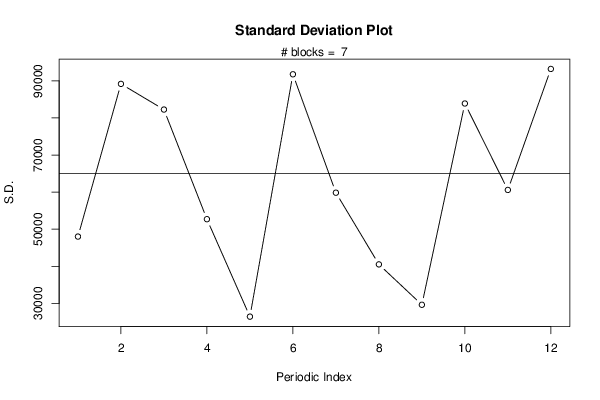
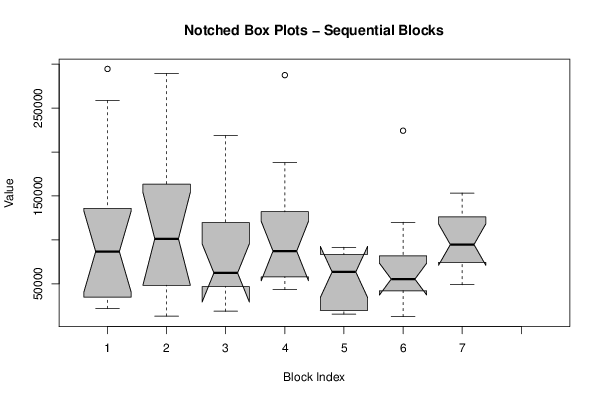
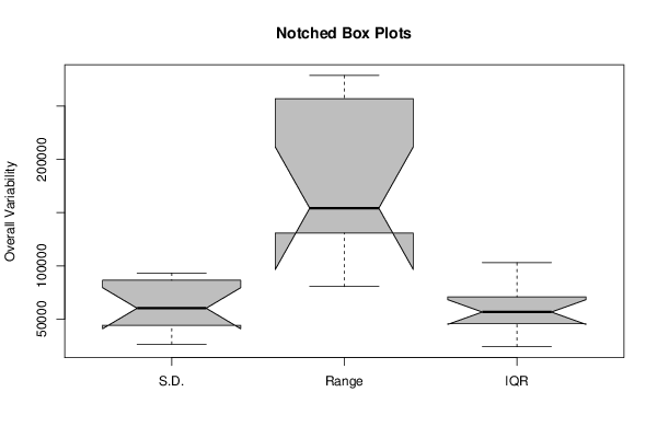
| Title produced by software | Standard Deviation Plot | ||||||||||||||||||||
| Date of computation | Wed, 28 Nov 2012 13:29:39 -0500 | ||||||||||||||||||||
| Cite this page as follows | Statistical Computations at FreeStatistics.org, Office for Research Development and Education, URL https://freestatistics.org/blog/index.php?v=date/2012/Nov/28/t1354127514hkojpiawgdzvxle.htm/, Retrieved Thu, 25 Apr 2024 00:49:06 +0000 | ||||||||||||||||||||
| Statistical Computations at FreeStatistics.org, Office for Research Development and Education, URL https://freestatistics.org/blog/index.php?pk=194208, Retrieved Thu, 25 Apr 2024 00:49:06 +0000 | |||||||||||||||||||||
| QR Codes: | |||||||||||||||||||||
|
| |||||||||||||||||||||
| Original text written by user: | |||||||||||||||||||||
| IsPrivate? | No (this computation is public) | ||||||||||||||||||||
| User-defined keywords | |||||||||||||||||||||
| Estimated Impact | 100 | ||||||||||||||||||||
Tree of Dependent Computations | |||||||||||||||||||||
| Family? (F = Feedback message, R = changed R code, M = changed R Module, P = changed Parameters, D = changed Data) | |||||||||||||||||||||
| - [Standard Deviation-Mean Plot] [inschrijving nieu...] [2012-11-28 18:22:24] [6e17e56f9bbdc65ea77b7e28bc808fc4] - RM D [Standard Deviation Plot] [verkoop aantal pr...] [2012-11-28 18:29:39] [32426a9b6b43a24d932e8bdfe421cad9] [Current] | |||||||||||||||||||||
| Feedback Forum | |||||||||||||||||||||
Post a new message | |||||||||||||||||||||
Dataset | |||||||||||||||||||||
| Dataseries X: | |||||||||||||||||||||
124275 58605 21828 42811 65963 128457 26867 143540 107458 258558 22475 294584 159848 289458 117950 78351 84589 44324 52285 185486 23846 13257 166999 148488 74747 55700 218584 187888 44788 18840 48787 69100 41892 90588 148574 50201 86828 102785 118844 145288 56790 287525 187880 87740 55258 58769 43366 77051 91574 15533 18425 65192 81059 73322 91261 86166 61842 25192 21059 15855 12618 101667 224275 55700 60748 41848 61781 120077 42032 46485 36861 55027 48999 68352 126987 86526 125340 69029 153287 135724 92108 119906 79798 97206 | |||||||||||||||||||||
Tables (Output of Computation) | |||||||||||||||||||||
| |||||||||||||||||||||
Figures (Output of Computation) | |||||||||||||||||||||
Input Parameters & R Code | |||||||||||||||||||||
| Parameters (Session): | |||||||||||||||||||||
| par1 = 12 ; | |||||||||||||||||||||
| Parameters (R input): | |||||||||||||||||||||
| par1 = 12 ; | |||||||||||||||||||||
| R code (references can be found in the software module): | |||||||||||||||||||||
par1 <- as.numeric(par1) | |||||||||||||||||||||