Free Statistics
of Irreproducible Research!
Description of Statistical Computation | |||||||||||||||||||||||||||||||||||||||||||||||||||||||||||||||||||||||||||||||||||||||||||||||||||||||||||||||||||||||||||||||||||||||||||||||||||||||||||||||||||||||||||||||||||||||||||||||||||||||||||||||||||||||||||||||||||||||||||||||||||||||||||||||||||||||||||||||||||||||||||||||||||||||||||||||||||||||||||||||||||||||||||||||||||||||||||||||||||||||||||||||||||||||||||||||||
|---|---|---|---|---|---|---|---|---|---|---|---|---|---|---|---|---|---|---|---|---|---|---|---|---|---|---|---|---|---|---|---|---|---|---|---|---|---|---|---|---|---|---|---|---|---|---|---|---|---|---|---|---|---|---|---|---|---|---|---|---|---|---|---|---|---|---|---|---|---|---|---|---|---|---|---|---|---|---|---|---|---|---|---|---|---|---|---|---|---|---|---|---|---|---|---|---|---|---|---|---|---|---|---|---|---|---|---|---|---|---|---|---|---|---|---|---|---|---|---|---|---|---|---|---|---|---|---|---|---|---|---|---|---|---|---|---|---|---|---|---|---|---|---|---|---|---|---|---|---|---|---|---|---|---|---|---|---|---|---|---|---|---|---|---|---|---|---|---|---|---|---|---|---|---|---|---|---|---|---|---|---|---|---|---|---|---|---|---|---|---|---|---|---|---|---|---|---|---|---|---|---|---|---|---|---|---|---|---|---|---|---|---|---|---|---|---|---|---|---|---|---|---|---|---|---|---|---|---|---|---|---|---|---|---|---|---|---|---|---|---|---|---|---|---|---|---|---|---|---|---|---|---|---|---|---|---|---|---|---|---|---|---|---|---|---|---|---|---|---|---|---|---|---|---|---|---|---|---|---|---|---|---|---|---|---|---|---|---|---|---|---|---|---|---|---|---|---|---|---|---|---|---|---|---|---|---|---|---|---|---|---|---|---|---|---|---|---|---|---|---|---|---|---|---|---|---|---|---|---|---|---|---|---|---|---|---|---|---|---|---|---|---|---|---|---|---|---|---|---|---|---|---|---|---|---|---|---|---|---|---|---|---|---|---|---|---|---|---|---|---|---|---|---|---|---|---|---|---|---|---|---|---|---|---|---|
| Author's title | |||||||||||||||||||||||||||||||||||||||||||||||||||||||||||||||||||||||||||||||||||||||||||||||||||||||||||||||||||||||||||||||||||||||||||||||||||||||||||||||||||||||||||||||||||||||||||||||||||||||||||||||||||||||||||||||||||||||||||||||||||||||||||||||||||||||||||||||||||||||||||||||||||||||||||||||||||||||||||||||||||||||||||||||||||||||||||||||||||||||||||||||||||||||||||||||||
| Author | *The author of this computation has been verified* | ||||||||||||||||||||||||||||||||||||||||||||||||||||||||||||||||||||||||||||||||||||||||||||||||||||||||||||||||||||||||||||||||||||||||||||||||||||||||||||||||||||||||||||||||||||||||||||||||||||||||||||||||||||||||||||||||||||||||||||||||||||||||||||||||||||||||||||||||||||||||||||||||||||||||||||||||||||||||||||||||||||||||||||||||||||||||||||||||||||||||||||||||||||||||||||||||
| R Software Module | rwasp_pairs.wasp | ||||||||||||||||||||||||||||||||||||||||||||||||||||||||||||||||||||||||||||||||||||||||||||||||||||||||||||||||||||||||||||||||||||||||||||||||||||||||||||||||||||||||||||||||||||||||||||||||||||||||||||||||||||||||||||||||||||||||||||||||||||||||||||||||||||||||||||||||||||||||||||||||||||||||||||||||||||||||||||||||||||||||||||||||||||||||||||||||||||||||||||||||||||||||||||||||
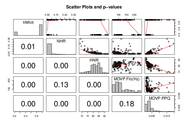
| Title produced by software | Kendall tau Correlation Matrix | ||||||||||||||||||||||||||||||||||||||||||||||||||||||||||||||||||||||||||||||||||||||||||||||||||||||||||||||||||||||||||||||||||||||||||||||||||||||||||||||||||||||||||||||||||||||||||||||||||||||||||||||||||||||||||||||||||||||||||||||||||||||||||||||||||||||||||||||||||||||||||||||||||||||||||||||||||||||||||||||||||||||||||||||||||||||||||||||||||||||||||||||||||||||||||||||||
| Date of computation | Thu, 05 Dec 2013 14:48:06 -0500 | ||||||||||||||||||||||||||||||||||||||||||||||||||||||||||||||||||||||||||||||||||||||||||||||||||||||||||||||||||||||||||||||||||||||||||||||||||||||||||||||||||||||||||||||||||||||||||||||||||||||||||||||||||||||||||||||||||||||||||||||||||||||||||||||||||||||||||||||||||||||||||||||||||||||||||||||||||||||||||||||||||||||||||||||||||||||||||||||||||||||||||||||||||||||||||||||||
| Cite this page as follows | Statistical Computations at FreeStatistics.org, Office for Research Development and Education, URL https://freestatistics.org/blog/index.php?v=date/2013/Dec/05/t1386272957556z2u6k6273jnq.htm/, Retrieved Sat, 20 Apr 2024 07:01:01 +0000 | ||||||||||||||||||||||||||||||||||||||||||||||||||||||||||||||||||||||||||||||||||||||||||||||||||||||||||||||||||||||||||||||||||||||||||||||||||||||||||||||||||||||||||||||||||||||||||||||||||||||||||||||||||||||||||||||||||||||||||||||||||||||||||||||||||||||||||||||||||||||||||||||||||||||||||||||||||||||||||||||||||||||||||||||||||||||||||||||||||||||||||||||||||||||||||||||||
| Statistical Computations at FreeStatistics.org, Office for Research Development and Education, URL https://freestatistics.org/blog/index.php?pk=231231, Retrieved Sat, 20 Apr 2024 07:01:01 +0000 | |||||||||||||||||||||||||||||||||||||||||||||||||||||||||||||||||||||||||||||||||||||||||||||||||||||||||||||||||||||||||||||||||||||||||||||||||||||||||||||||||||||||||||||||||||||||||||||||||||||||||||||||||||||||||||||||||||||||||||||||||||||||||||||||||||||||||||||||||||||||||||||||||||||||||||||||||||||||||||||||||||||||||||||||||||||||||||||||||||||||||||||||||||||||||||||||||
| QR Codes: | |||||||||||||||||||||||||||||||||||||||||||||||||||||||||||||||||||||||||||||||||||||||||||||||||||||||||||||||||||||||||||||||||||||||||||||||||||||||||||||||||||||||||||||||||||||||||||||||||||||||||||||||||||||||||||||||||||||||||||||||||||||||||||||||||||||||||||||||||||||||||||||||||||||||||||||||||||||||||||||||||||||||||||||||||||||||||||||||||||||||||||||||||||||||||||||||||
|
| |||||||||||||||||||||||||||||||||||||||||||||||||||||||||||||||||||||||||||||||||||||||||||||||||||||||||||||||||||||||||||||||||||||||||||||||||||||||||||||||||||||||||||||||||||||||||||||||||||||||||||||||||||||||||||||||||||||||||||||||||||||||||||||||||||||||||||||||||||||||||||||||||||||||||||||||||||||||||||||||||||||||||||||||||||||||||||||||||||||||||||||||||||||||||||||||||
| Original text written by user: | |||||||||||||||||||||||||||||||||||||||||||||||||||||||||||||||||||||||||||||||||||||||||||||||||||||||||||||||||||||||||||||||||||||||||||||||||||||||||||||||||||||||||||||||||||||||||||||||||||||||||||||||||||||||||||||||||||||||||||||||||||||||||||||||||||||||||||||||||||||||||||||||||||||||||||||||||||||||||||||||||||||||||||||||||||||||||||||||||||||||||||||||||||||||||||||||||
| IsPrivate? | No (this computation is public) | ||||||||||||||||||||||||||||||||||||||||||||||||||||||||||||||||||||||||||||||||||||||||||||||||||||||||||||||||||||||||||||||||||||||||||||||||||||||||||||||||||||||||||||||||||||||||||||||||||||||||||||||||||||||||||||||||||||||||||||||||||||||||||||||||||||||||||||||||||||||||||||||||||||||||||||||||||||||||||||||||||||||||||||||||||||||||||||||||||||||||||||||||||||||||||||||||
| User-defined keywords | |||||||||||||||||||||||||||||||||||||||||||||||||||||||||||||||||||||||||||||||||||||||||||||||||||||||||||||||||||||||||||||||||||||||||||||||||||||||||||||||||||||||||||||||||||||||||||||||||||||||||||||||||||||||||||||||||||||||||||||||||||||||||||||||||||||||||||||||||||||||||||||||||||||||||||||||||||||||||||||||||||||||||||||||||||||||||||||||||||||||||||||||||||||||||||||||||
| Estimated Impact | 48 | ||||||||||||||||||||||||||||||||||||||||||||||||||||||||||||||||||||||||||||||||||||||||||||||||||||||||||||||||||||||||||||||||||||||||||||||||||||||||||||||||||||||||||||||||||||||||||||||||||||||||||||||||||||||||||||||||||||||||||||||||||||||||||||||||||||||||||||||||||||||||||||||||||||||||||||||||||||||||||||||||||||||||||||||||||||||||||||||||||||||||||||||||||||||||||||||||
Tree of Dependent Computations | |||||||||||||||||||||||||||||||||||||||||||||||||||||||||||||||||||||||||||||||||||||||||||||||||||||||||||||||||||||||||||||||||||||||||||||||||||||||||||||||||||||||||||||||||||||||||||||||||||||||||||||||||||||||||||||||||||||||||||||||||||||||||||||||||||||||||||||||||||||||||||||||||||||||||||||||||||||||||||||||||||||||||||||||||||||||||||||||||||||||||||||||||||||||||||||||||
| Family? (F = Feedback message, R = changed R code, M = changed R Module, P = changed Parameters, D = changed Data) | |||||||||||||||||||||||||||||||||||||||||||||||||||||||||||||||||||||||||||||||||||||||||||||||||||||||||||||||||||||||||||||||||||||||||||||||||||||||||||||||||||||||||||||||||||||||||||||||||||||||||||||||||||||||||||||||||||||||||||||||||||||||||||||||||||||||||||||||||||||||||||||||||||||||||||||||||||||||||||||||||||||||||||||||||||||||||||||||||||||||||||||||||||||||||||||||||
| - [Kendall tau Correlation Matrix] [] [2013-12-05 19:48:06] [02b53344bfc7e15f5310bf5039e578c4] [Current] | |||||||||||||||||||||||||||||||||||||||||||||||||||||||||||||||||||||||||||||||||||||||||||||||||||||||||||||||||||||||||||||||||||||||||||||||||||||||||||||||||||||||||||||||||||||||||||||||||||||||||||||||||||||||||||||||||||||||||||||||||||||||||||||||||||||||||||||||||||||||||||||||||||||||||||||||||||||||||||||||||||||||||||||||||||||||||||||||||||||||||||||||||||||||||||||||||
| Feedback Forum | |||||||||||||||||||||||||||||||||||||||||||||||||||||||||||||||||||||||||||||||||||||||||||||||||||||||||||||||||||||||||||||||||||||||||||||||||||||||||||||||||||||||||||||||||||||||||||||||||||||||||||||||||||||||||||||||||||||||||||||||||||||||||||||||||||||||||||||||||||||||||||||||||||||||||||||||||||||||||||||||||||||||||||||||||||||||||||||||||||||||||||||||||||||||||||||||||
Post a new message | |||||||||||||||||||||||||||||||||||||||||||||||||||||||||||||||||||||||||||||||||||||||||||||||||||||||||||||||||||||||||||||||||||||||||||||||||||||||||||||||||||||||||||||||||||||||||||||||||||||||||||||||||||||||||||||||||||||||||||||||||||||||||||||||||||||||||||||||||||||||||||||||||||||||||||||||||||||||||||||||||||||||||||||||||||||||||||||||||||||||||||||||||||||||||||||||||
Dataset | |||||||||||||||||||||||||||||||||||||||||||||||||||||||||||||||||||||||||||||||||||||||||||||||||||||||||||||||||||||||||||||||||||||||||||||||||||||||||||||||||||||||||||||||||||||||||||||||||||||||||||||||||||||||||||||||||||||||||||||||||||||||||||||||||||||||||||||||||||||||||||||||||||||||||||||||||||||||||||||||||||||||||||||||||||||||||||||||||||||||||||||||||||||||||||||||||
| Dataseries X: | |||||||||||||||||||||||||||||||||||||||||||||||||||||||||||||||||||||||||||||||||||||||||||||||||||||||||||||||||||||||||||||||||||||||||||||||||||||||||||||||||||||||||||||||||||||||||||||||||||||||||||||||||||||||||||||||||||||||||||||||||||||||||||||||||||||||||||||||||||||||||||||||||||||||||||||||||||||||||||||||||||||||||||||||||||||||||||||||||||||||||||||||||||||||||||||||||
1 0.02211 21.033 74.997 0.00554 1 0.01929 19.085 113.819 0.00696 1 0.01309 20.651 111.555 0.00781 1 0.01353 20.644 111.366 0.00698 1 0.01767 19.649 110.655 0.00908 1 0.01222 21.378 113.787 0.0075 1 0.00607 24.886 114.82 0.00202 1 0.00344 26.892 104.315 0.00182 1 0.0107 21.812 91.754 0.00332 1 0.01022 21.862 91.226 0.00332 1 0.01166 21.118 84.072 0.0033 1 0.01141 21.414 86.292 0.00336 1 0.00581 25.703 131.276 0.00153 1 0.01041 24.889 76.556 0.00208 1 0.00609 24.922 75.836 0.00149 1 0.00839 25.175 83.159 0.00203 1 0.01859 22.333 82.764 0.00292 1 0.02919 20.376 75.603 0.00387 1 0.0316 17.28 68.623 0.00432 1 0.03365 17.153 142.822 0.00399 1 0.03871 17.536 65.782 0.0045 1 0.01849 19.493 78.128 0.00267 1 0.0128 22.468 79.068 0.00247 1 0.0184 20.422 86.18 0.00258 1 0.01778 23.831 76.779 0.0039 1 0.02887 22.066 77.968 0.00375 1 0.01095 25.908 75.501 0.00234 1 0.01328 25.119 81.737 0.00275 1 0.00677 25.97 80.055 0.00176 1 0.0117 25.678 77.63 0.00253 0 0.00339 26.775 192.055 0.00168 0 0.00167 30.94 192.091 0.00138 0 0.00119 30.775 193.104 0.00135 0 0.00072 32.684 197.079 0.00107 0 0.00065 33.047 196.16 0.00106 0 0.00135 31.732 195.708 0.00115 1 0.00586 23.216 168.013 0.00241 1 0.0034 24.951 163.564 0.00218 1 0.00231 26.738 175.456 0.00166 1 0.00265 26.31 173.015 0.00182 1 0.00231 26.822 177.584 0.00175 1 0.00257 26.453 166.977 0.00147 0 0.0074 22.736 225.227 0.00182 0 0.00675 23.145 232.483 0.00173 0 0.00454 25.368 232.435 0.00137 0 0.00476 25.032 227.911 0.00139 0 0.00476 24.602 231.848 0.00148 0 0.00432 26.805 182.786 0.00113 0 0.00839 23.162 115.765 0.00203 0 0.00462 24.971 114.676 0.00155 0 0.00479 25.135 117.495 0.00167 0 0.00474 25.03 112.773 0.00169 0 0.00481 24.692 122.08 0.00166 0 0.00484 25.429 118.604 0.00183 1 0.01036 21.028 102.874 0.00486 1 0.0118 20.767 104.437 0.00539 1 0.00969 21.422 103.37 0.00514 1 0.00681 22.817 110.402 0.00469 1 0.00786 22.603 108.153 0.00493 1 0.01143 21.66 104.68 0.0052 0 0.00871 25.554 109.379 0.00152 0 0.00301 26.138 98.664 0.00151 0 0.0034 25.856 205.495 0.00144 0 0.00351 25.964 223.634 0.00155 0 0.003 26.415 221.156 0.00113 0 0.0042 24.547 113.201 0.0014 1 0.02183 19.56 67.021 0.0044 1 0.02659 19.979 66.004 0.00463 1 0.04882 20.338 65.809 0.00467 1 0.02431 21.718 67.343 0.00354 1 0.02599 20.264 65.476 0.00419 1 0.03361 18.57 65.75 0.00478 1 0.00442 25.742 111.208 0.0022 1 0.00623 24.178 107.024 0.00329 1 0.00479 25.438 107.316 0.00283 1 0.00472 25.197 105.007 0.00289 1 0.00905 23.37 106.981 0.00289 1 0.0042 25.82 106.821 0.0028 1 0.01062 21.875 90.264 0.00332 1 0.0222 19.2 85.545 0.00576 1 0.01823 19.055 84.51 0.00415 1 0.01825 19.659 87.549 0.00371 1 0.01237 20.536 95.628 0.00348 1 0.00882 22.244 87.804 0.00258 1 0.0547 13.893 75.344 0.0042 1 0.02782 16.176 155.495 0.00244 1 0.03151 15.924 141.047 0.00194 1 0.04824 13.922 125.61 0.00312 1 0.04214 14.739 74.677 0.00254 1 0.07223 11.866 144.878 0.00419 1 0.08725 11.744 78.032 0.00453 1 0.01658 19.664 147.226 0.00227 1 0.01914 18.78 142.299 0.00256 1 0.01211 20.969 76.596 0.00226 1 0.0085 22.219 68.401 0.00196 1 0.01018 21.693 149.605 0.00197 1 0.00852 22.663 144.811 0.00184 1 0.08151 15.338 116.187 0.00623 1 0.10323 15.433 96.206 0.00655 1 0.16744 12.435 99.77 0.0099 1 0.31482 8.867 116.346 0.01522 1 0.11843 15.06 75.632 0.00909 1 0.2593 10.489 66.157 0.01628 1 0.00495 26.759 75.349 0.00136 1 0.00243 28.409 128.621 0.001 1 0.00578 27.421 133.608 0.00134 1 0.00233 29.746 144.148 0.00092 1 0.00659 26.833 133.751 0.00122 1 0.00238 29.928 132.857 0.00096 1 0.00947 21.934 80.297 0.00389 1 0.00704 23.239 89.686 0.00337 1 0.0083 22.407 199.02 0.00339 1 0.01316 21.305 189.621 0.00485 1 0.0062 23.671 185.258 0.0028 1 0.01048 21.864 92.02 0.00246 1 0.06051 23.693 69.085 0.00385 1 0.01554 26.356 71.948 0.00207 1 0.01802 25.69 79.032 0.00261 1 0.00856 25.02 82.063 0.00194 1 0.00681 24.581 93.978 0.00128 1 0.0235 24.743 88.251 0.00314 1 0.01161 27.166 83.961 0.00221 1 0.01968 18.305 83.34 0.00398 1 0.01813 18.784 79.187 0.00449 1 0.0202 19.196 79.82 0.00395 1 0.01874 18.857 80.637 0.00422 1 0.01794 18.178 81.114 0.00327 1 0.01796 18.33 79.512 0.00351 1 0.01724 26.842 109.216 0.00192 1 0.00487 26.369 105.667 0.00135 1 0.0161 23.949 100.209 0.00238 1 0.01015 26.017 104.773 0.00205 1 0.00903 23.389 86.795 0.0017 1 0.00504 25.619 109.836 0.00171 1 0.03031 17.06 93.105 0.00319 1 0.02529 17.707 105.554 0.00315 1 0.02278 19.013 107.816 0.00283 1 0.0369 16.747 100.673 0.00312 1 0.02629 17.366 104.095 0.0029 1 0.01827 18.801 109.815 0.00232 1 0.02485 18.54 79.543 0.00269 1 0.04238 15.648 91.802 0.00428 1 0.01728 18.702 148.691 0.00215 1 0.0201 18.687 86.232 0.00211 1 0.01049 20.68 164.168 0.00133 1 0.01493 20.366 87.638 0.00188 1 0.0753 12.359 151.451 0.00946 1 0.06057 14.367 161.34 0.00819 1 0.08069 12.298 165.982 0.01027 1 0.07889 14.989 177.258 0.00963 1 0.10952 12.529 149.442 0.01154 1 0.21713 8.441 168.793 0.01958 1 0.16265 9.449 174.478 0.01699 1 0.04179 21.52 98.25 0.00332 1 0.04611 21.824 88.833 0.003 1 0.02631 22.431 95.654 0.003 1 0.03191 22.953 94.794 0.00339 1 0.10748 19.075 100.757 0.00718 1 0.03828 21.534 97.543 0.00454 1 0.02663 19.651 112.173 0.00318 1 0.02073 20.437 77.022 0.00316 1 0.0281 19.388 107.802 0.00329 1 0.02707 18.954 91.121 0.0034 1 0.01435 21.219 97.527 0.00284 1 0.03882 18.447 85.902 0.00461 0 0.0062 24.078 102.137 0.00153 0 0.00533 24.679 229.256 0.00159 0 0.0091 21.083 237.303 0.00186 0 0.01337 19.269 90.794 0.00448 0 0.00965 21.02 219.783 0.00283 0 0.01049 21.528 239.17 0.00237 0 0.00435 26.436 105.715 0.0019 0 0.0043 26.55 100.139 0.002 0 0.00478 26.547 96.913 0.00203 0 0.0059 25.445 99.923 0.00218 0 0.00401 26.005 108.634 0.00199 0 0.00415 26.143 108.97 0.00213 1 0.0057 24.151 129.859 0.00162 1 0.00488 24.412 138.99 0.00186 1 0.0054 23.683 135.041 0.00231 1 0.00611 23.133 144.736 0.00233 1 0.00639 22.866 141.998 0.00235 1 0.00595 23.008 144.786 0.00198 0 0.00955 23.079 106.656 0.0027 0 0.01179 22.085 99.503 0.00346 0 0.00737 24.199 96.983 0.00192 0 0.01397 23.958 86.228 0.00263 0 0.0068 25.023 94.246 0.00148 0 0.00703 24.775 86.647 0.00184 0 0.04441 19.368 78.228 0.00396 0 0.02764 19.517 94.261 0.00259 0 0.0181 19.147 89.488 0.00292 0 0.10715 17.883 74.287 0.00564 0 0.07223 19.02 74.904 0.0039 0 0.04398 21.209 77.973 0.00317 | |||||||||||||||||||||||||||||||||||||||||||||||||||||||||||||||||||||||||||||||||||||||||||||||||||||||||||||||||||||||||||||||||||||||||||||||||||||||||||||||||||||||||||||||||||||||||||||||||||||||||||||||||||||||||||||||||||||||||||||||||||||||||||||||||||||||||||||||||||||||||||||||||||||||||||||||||||||||||||||||||||||||||||||||||||||||||||||||||||||||||||||||||||||||||||||||||
Tables (Output of Computation) | |||||||||||||||||||||||||||||||||||||||||||||||||||||||||||||||||||||||||||||||||||||||||||||||||||||||||||||||||||||||||||||||||||||||||||||||||||||||||||||||||||||||||||||||||||||||||||||||||||||||||||||||||||||||||||||||||||||||||||||||||||||||||||||||||||||||||||||||||||||||||||||||||||||||||||||||||||||||||||||||||||||||||||||||||||||||||||||||||||||||||||||||||||||||||||||||||
| |||||||||||||||||||||||||||||||||||||||||||||||||||||||||||||||||||||||||||||||||||||||||||||||||||||||||||||||||||||||||||||||||||||||||||||||||||||||||||||||||||||||||||||||||||||||||||||||||||||||||||||||||||||||||||||||||||||||||||||||||||||||||||||||||||||||||||||||||||||||||||||||||||||||||||||||||||||||||||||||||||||||||||||||||||||||||||||||||||||||||||||||||||||||||||||||||
Figures (Output of Computation) | |||||||||||||||||||||||||||||||||||||||||||||||||||||||||||||||||||||||||||||||||||||||||||||||||||||||||||||||||||||||||||||||||||||||||||||||||||||||||||||||||||||||||||||||||||||||||||||||||||||||||||||||||||||||||||||||||||||||||||||||||||||||||||||||||||||||||||||||||||||||||||||||||||||||||||||||||||||||||||||||||||||||||||||||||||||||||||||||||||||||||||||||||||||||||||||||||
Input Parameters & R Code | |||||||||||||||||||||||||||||||||||||||||||||||||||||||||||||||||||||||||||||||||||||||||||||||||||||||||||||||||||||||||||||||||||||||||||||||||||||||||||||||||||||||||||||||||||||||||||||||||||||||||||||||||||||||||||||||||||||||||||||||||||||||||||||||||||||||||||||||||||||||||||||||||||||||||||||||||||||||||||||||||||||||||||||||||||||||||||||||||||||||||||||||||||||||||||||||||
| Parameters (Session): | |||||||||||||||||||||||||||||||||||||||||||||||||||||||||||||||||||||||||||||||||||||||||||||||||||||||||||||||||||||||||||||||||||||||||||||||||||||||||||||||||||||||||||||||||||||||||||||||||||||||||||||||||||||||||||||||||||||||||||||||||||||||||||||||||||||||||||||||||||||||||||||||||||||||||||||||||||||||||||||||||||||||||||||||||||||||||||||||||||||||||||||||||||||||||||||||||
| par1 = pearson ; | |||||||||||||||||||||||||||||||||||||||||||||||||||||||||||||||||||||||||||||||||||||||||||||||||||||||||||||||||||||||||||||||||||||||||||||||||||||||||||||||||||||||||||||||||||||||||||||||||||||||||||||||||||||||||||||||||||||||||||||||||||||||||||||||||||||||||||||||||||||||||||||||||||||||||||||||||||||||||||||||||||||||||||||||||||||||||||||||||||||||||||||||||||||||||||||||||
| Parameters (R input): | |||||||||||||||||||||||||||||||||||||||||||||||||||||||||||||||||||||||||||||||||||||||||||||||||||||||||||||||||||||||||||||||||||||||||||||||||||||||||||||||||||||||||||||||||||||||||||||||||||||||||||||||||||||||||||||||||||||||||||||||||||||||||||||||||||||||||||||||||||||||||||||||||||||||||||||||||||||||||||||||||||||||||||||||||||||||||||||||||||||||||||||||||||||||||||||||||
| par1 = pearson ; | |||||||||||||||||||||||||||||||||||||||||||||||||||||||||||||||||||||||||||||||||||||||||||||||||||||||||||||||||||||||||||||||||||||||||||||||||||||||||||||||||||||||||||||||||||||||||||||||||||||||||||||||||||||||||||||||||||||||||||||||||||||||||||||||||||||||||||||||||||||||||||||||||||||||||||||||||||||||||||||||||||||||||||||||||||||||||||||||||||||||||||||||||||||||||||||||||
| R code (references can be found in the software module): | |||||||||||||||||||||||||||||||||||||||||||||||||||||||||||||||||||||||||||||||||||||||||||||||||||||||||||||||||||||||||||||||||||||||||||||||||||||||||||||||||||||||||||||||||||||||||||||||||||||||||||||||||||||||||||||||||||||||||||||||||||||||||||||||||||||||||||||||||||||||||||||||||||||||||||||||||||||||||||||||||||||||||||||||||||||||||||||||||||||||||||||||||||||||||||||||||
panel.tau <- function(x, y, digits=2, prefix='', cex.cor) | |||||||||||||||||||||||||||||||||||||||||||||||||||||||||||||||||||||||||||||||||||||||||||||||||||||||||||||||||||||||||||||||||||||||||||||||||||||||||||||||||||||||||||||||||||||||||||||||||||||||||||||||||||||||||||||||||||||||||||||||||||||||||||||||||||||||||||||||||||||||||||||||||||||||||||||||||||||||||||||||||||||||||||||||||||||||||||||||||||||||||||||||||||||||||||||||||