Free Statistics
of Irreproducible Research!
Description of Statistical Computation | |||||||||||||||||||||||||||||||||||||||||||||||||||||||||||||||||||||||||||||||||||||||||||||||||||||||||||||||||||||||||||||||||||||||||||||||||||||||||||||||||||||||||||||||||||||||||||||||||||||||||||||||||||||||||||||||||||||||||||||||||||||||||||||||||||||||||||||||||||||||||||||||||||||||||||||||||||||||||||||||||||||||||||||||||||||||||||||||||||||||||||||||||||||||||||||||||||||||||||||||||||||||||||||||||||||||||||||||||||||||||||||||||||||||||||||||||||||||||||||||||||||||||||||
|---|---|---|---|---|---|---|---|---|---|---|---|---|---|---|---|---|---|---|---|---|---|---|---|---|---|---|---|---|---|---|---|---|---|---|---|---|---|---|---|---|---|---|---|---|---|---|---|---|---|---|---|---|---|---|---|---|---|---|---|---|---|---|---|---|---|---|---|---|---|---|---|---|---|---|---|---|---|---|---|---|---|---|---|---|---|---|---|---|---|---|---|---|---|---|---|---|---|---|---|---|---|---|---|---|---|---|---|---|---|---|---|---|---|---|---|---|---|---|---|---|---|---|---|---|---|---|---|---|---|---|---|---|---|---|---|---|---|---|---|---|---|---|---|---|---|---|---|---|---|---|---|---|---|---|---|---|---|---|---|---|---|---|---|---|---|---|---|---|---|---|---|---|---|---|---|---|---|---|---|---|---|---|---|---|---|---|---|---|---|---|---|---|---|---|---|---|---|---|---|---|---|---|---|---|---|---|---|---|---|---|---|---|---|---|---|---|---|---|---|---|---|---|---|---|---|---|---|---|---|---|---|---|---|---|---|---|---|---|---|---|---|---|---|---|---|---|---|---|---|---|---|---|---|---|---|---|---|---|---|---|---|---|---|---|---|---|---|---|---|---|---|---|---|---|---|---|---|---|---|---|---|---|---|---|---|---|---|---|---|---|---|---|---|---|---|---|---|---|---|---|---|---|---|---|---|---|---|---|---|---|---|---|---|---|---|---|---|---|---|---|---|---|---|---|---|---|---|---|---|---|---|---|---|---|---|---|---|---|---|---|---|---|---|---|---|---|---|---|---|---|---|---|---|---|---|---|---|---|---|---|---|---|---|---|---|---|---|---|---|---|---|---|---|---|---|---|---|---|---|---|---|---|---|---|---|---|---|---|---|---|---|---|---|---|---|---|---|---|---|---|---|---|---|---|---|---|---|---|---|---|---|---|---|---|---|---|---|---|---|---|---|---|---|---|---|---|---|---|---|---|---|---|---|---|---|---|---|---|---|---|---|---|---|---|---|---|---|---|---|---|---|---|---|---|---|---|---|---|---|---|---|---|---|---|---|---|---|---|---|---|---|---|---|---|---|---|---|---|---|---|---|---|---|---|---|---|---|---|---|---|---|---|---|
| Author's title | |||||||||||||||||||||||||||||||||||||||||||||||||||||||||||||||||||||||||||||||||||||||||||||||||||||||||||||||||||||||||||||||||||||||||||||||||||||||||||||||||||||||||||||||||||||||||||||||||||||||||||||||||||||||||||||||||||||||||||||||||||||||||||||||||||||||||||||||||||||||||||||||||||||||||||||||||||||||||||||||||||||||||||||||||||||||||||||||||||||||||||||||||||||||||||||||||||||||||||||||||||||||||||||||||||||||||||||||||||||||||||||||||||||||||||||||||||||||||||||||||||||||||||||
| Author | *The author of this computation has been verified* | ||||||||||||||||||||||||||||||||||||||||||||||||||||||||||||||||||||||||||||||||||||||||||||||||||||||||||||||||||||||||||||||||||||||||||||||||||||||||||||||||||||||||||||||||||||||||||||||||||||||||||||||||||||||||||||||||||||||||||||||||||||||||||||||||||||||||||||||||||||||||||||||||||||||||||||||||||||||||||||||||||||||||||||||||||||||||||||||||||||||||||||||||||||||||||||||||||||||||||||||||||||||||||||||||||||||||||||||||||||||||||||||||||||||||||||||||||||||||||||||||||||||||||||
| R Software Module | rwasp_pairs.wasp | ||||||||||||||||||||||||||||||||||||||||||||||||||||||||||||||||||||||||||||||||||||||||||||||||||||||||||||||||||||||||||||||||||||||||||||||||||||||||||||||||||||||||||||||||||||||||||||||||||||||||||||||||||||||||||||||||||||||||||||||||||||||||||||||||||||||||||||||||||||||||||||||||||||||||||||||||||||||||||||||||||||||||||||||||||||||||||||||||||||||||||||||||||||||||||||||||||||||||||||||||||||||||||||||||||||||||||||||||||||||||||||||||||||||||||||||||||||||||||||||||||||||||||||
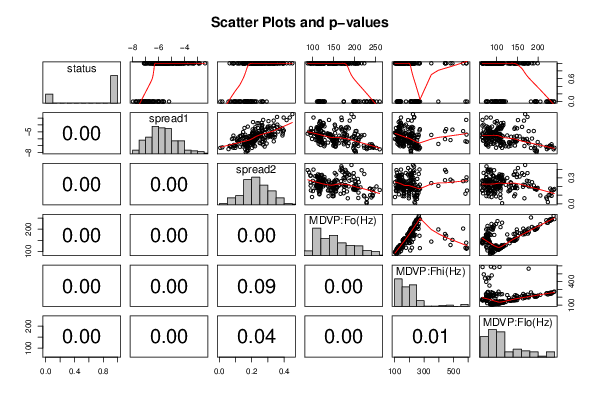
| Title produced by software | Kendall tau Correlation Matrix | ||||||||||||||||||||||||||||||||||||||||||||||||||||||||||||||||||||||||||||||||||||||||||||||||||||||||||||||||||||||||||||||||||||||||||||||||||||||||||||||||||||||||||||||||||||||||||||||||||||||||||||||||||||||||||||||||||||||||||||||||||||||||||||||||||||||||||||||||||||||||||||||||||||||||||||||||||||||||||||||||||||||||||||||||||||||||||||||||||||||||||||||||||||||||||||||||||||||||||||||||||||||||||||||||||||||||||||||||||||||||||||||||||||||||||||||||||||||||||||||||||||||||||||
| Date of computation | Wed, 11 Dec 2013 14:06:33 -0500 | ||||||||||||||||||||||||||||||||||||||||||||||||||||||||||||||||||||||||||||||||||||||||||||||||||||||||||||||||||||||||||||||||||||||||||||||||||||||||||||||||||||||||||||||||||||||||||||||||||||||||||||||||||||||||||||||||||||||||||||||||||||||||||||||||||||||||||||||||||||||||||||||||||||||||||||||||||||||||||||||||||||||||||||||||||||||||||||||||||||||||||||||||||||||||||||||||||||||||||||||||||||||||||||||||||||||||||||||||||||||||||||||||||||||||||||||||||||||||||||||||||||||||||||
| Cite this page as follows | Statistical Computations at FreeStatistics.org, Office for Research Development and Education, URL https://freestatistics.org/blog/index.php?v=date/2013/Dec/11/t1386788807g85g9d0t5lzfm80.htm/, Retrieved Thu, 18 Apr 2024 11:33:40 +0000 | ||||||||||||||||||||||||||||||||||||||||||||||||||||||||||||||||||||||||||||||||||||||||||||||||||||||||||||||||||||||||||||||||||||||||||||||||||||||||||||||||||||||||||||||||||||||||||||||||||||||||||||||||||||||||||||||||||||||||||||||||||||||||||||||||||||||||||||||||||||||||||||||||||||||||||||||||||||||||||||||||||||||||||||||||||||||||||||||||||||||||||||||||||||||||||||||||||||||||||||||||||||||||||||||||||||||||||||||||||||||||||||||||||||||||||||||||||||||||||||||||||||||||||||
| Statistical Computations at FreeStatistics.org, Office for Research Development and Education, URL https://freestatistics.org/blog/index.php?pk=232140, Retrieved Thu, 18 Apr 2024 11:33:40 +0000 | |||||||||||||||||||||||||||||||||||||||||||||||||||||||||||||||||||||||||||||||||||||||||||||||||||||||||||||||||||||||||||||||||||||||||||||||||||||||||||||||||||||||||||||||||||||||||||||||||||||||||||||||||||||||||||||||||||||||||||||||||||||||||||||||||||||||||||||||||||||||||||||||||||||||||||||||||||||||||||||||||||||||||||||||||||||||||||||||||||||||||||||||||||||||||||||||||||||||||||||||||||||||||||||||||||||||||||||||||||||||||||||||||||||||||||||||||||||||||||||||||||||||||||||
| QR Codes: | |||||||||||||||||||||||||||||||||||||||||||||||||||||||||||||||||||||||||||||||||||||||||||||||||||||||||||||||||||||||||||||||||||||||||||||||||||||||||||||||||||||||||||||||||||||||||||||||||||||||||||||||||||||||||||||||||||||||||||||||||||||||||||||||||||||||||||||||||||||||||||||||||||||||||||||||||||||||||||||||||||||||||||||||||||||||||||||||||||||||||||||||||||||||||||||||||||||||||||||||||||||||||||||||||||||||||||||||||||||||||||||||||||||||||||||||||||||||||||||||||||||||||||||
|
| |||||||||||||||||||||||||||||||||||||||||||||||||||||||||||||||||||||||||||||||||||||||||||||||||||||||||||||||||||||||||||||||||||||||||||||||||||||||||||||||||||||||||||||||||||||||||||||||||||||||||||||||||||||||||||||||||||||||||||||||||||||||||||||||||||||||||||||||||||||||||||||||||||||||||||||||||||||||||||||||||||||||||||||||||||||||||||||||||||||||||||||||||||||||||||||||||||||||||||||||||||||||||||||||||||||||||||||||||||||||||||||||||||||||||||||||||||||||||||||||||||||||||||||
| Original text written by user: | |||||||||||||||||||||||||||||||||||||||||||||||||||||||||||||||||||||||||||||||||||||||||||||||||||||||||||||||||||||||||||||||||||||||||||||||||||||||||||||||||||||||||||||||||||||||||||||||||||||||||||||||||||||||||||||||||||||||||||||||||||||||||||||||||||||||||||||||||||||||||||||||||||||||||||||||||||||||||||||||||||||||||||||||||||||||||||||||||||||||||||||||||||||||||||||||||||||||||||||||||||||||||||||||||||||||||||||||||||||||||||||||||||||||||||||||||||||||||||||||||||||||||||||
| IsPrivate? | No (this computation is public) | ||||||||||||||||||||||||||||||||||||||||||||||||||||||||||||||||||||||||||||||||||||||||||||||||||||||||||||||||||||||||||||||||||||||||||||||||||||||||||||||||||||||||||||||||||||||||||||||||||||||||||||||||||||||||||||||||||||||||||||||||||||||||||||||||||||||||||||||||||||||||||||||||||||||||||||||||||||||||||||||||||||||||||||||||||||||||||||||||||||||||||||||||||||||||||||||||||||||||||||||||||||||||||||||||||||||||||||||||||||||||||||||||||||||||||||||||||||||||||||||||||||||||||||
| User-defined keywords | |||||||||||||||||||||||||||||||||||||||||||||||||||||||||||||||||||||||||||||||||||||||||||||||||||||||||||||||||||||||||||||||||||||||||||||||||||||||||||||||||||||||||||||||||||||||||||||||||||||||||||||||||||||||||||||||||||||||||||||||||||||||||||||||||||||||||||||||||||||||||||||||||||||||||||||||||||||||||||||||||||||||||||||||||||||||||||||||||||||||||||||||||||||||||||||||||||||||||||||||||||||||||||||||||||||||||||||||||||||||||||||||||||||||||||||||||||||||||||||||||||||||||||||
| Estimated Impact | 71 | ||||||||||||||||||||||||||||||||||||||||||||||||||||||||||||||||||||||||||||||||||||||||||||||||||||||||||||||||||||||||||||||||||||||||||||||||||||||||||||||||||||||||||||||||||||||||||||||||||||||||||||||||||||||||||||||||||||||||||||||||||||||||||||||||||||||||||||||||||||||||||||||||||||||||||||||||||||||||||||||||||||||||||||||||||||||||||||||||||||||||||||||||||||||||||||||||||||||||||||||||||||||||||||||||||||||||||||||||||||||||||||||||||||||||||||||||||||||||||||||||||||||||||||
Tree of Dependent Computations | |||||||||||||||||||||||||||||||||||||||||||||||||||||||||||||||||||||||||||||||||||||||||||||||||||||||||||||||||||||||||||||||||||||||||||||||||||||||||||||||||||||||||||||||||||||||||||||||||||||||||||||||||||||||||||||||||||||||||||||||||||||||||||||||||||||||||||||||||||||||||||||||||||||||||||||||||||||||||||||||||||||||||||||||||||||||||||||||||||||||||||||||||||||||||||||||||||||||||||||||||||||||||||||||||||||||||||||||||||||||||||||||||||||||||||||||||||||||||||||||||||||||||||||
| Family? (F = Feedback message, R = changed R code, M = changed R Module, P = changed Parameters, D = changed Data) | |||||||||||||||||||||||||||||||||||||||||||||||||||||||||||||||||||||||||||||||||||||||||||||||||||||||||||||||||||||||||||||||||||||||||||||||||||||||||||||||||||||||||||||||||||||||||||||||||||||||||||||||||||||||||||||||||||||||||||||||||||||||||||||||||||||||||||||||||||||||||||||||||||||||||||||||||||||||||||||||||||||||||||||||||||||||||||||||||||||||||||||||||||||||||||||||||||||||||||||||||||||||||||||||||||||||||||||||||||||||||||||||||||||||||||||||||||||||||||||||||||||||||||||
| - [Kendall tau Correlation Matrix] [Workshop 10 Parki...] [2013-12-11 19:06:33] [9e345f4af24c955bbdd99e7ffb840b0f] [Current] | |||||||||||||||||||||||||||||||||||||||||||||||||||||||||||||||||||||||||||||||||||||||||||||||||||||||||||||||||||||||||||||||||||||||||||||||||||||||||||||||||||||||||||||||||||||||||||||||||||||||||||||||||||||||||||||||||||||||||||||||||||||||||||||||||||||||||||||||||||||||||||||||||||||||||||||||||||||||||||||||||||||||||||||||||||||||||||||||||||||||||||||||||||||||||||||||||||||||||||||||||||||||||||||||||||||||||||||||||||||||||||||||||||||||||||||||||||||||||||||||||||||||||||||
| Feedback Forum | |||||||||||||||||||||||||||||||||||||||||||||||||||||||||||||||||||||||||||||||||||||||||||||||||||||||||||||||||||||||||||||||||||||||||||||||||||||||||||||||||||||||||||||||||||||||||||||||||||||||||||||||||||||||||||||||||||||||||||||||||||||||||||||||||||||||||||||||||||||||||||||||||||||||||||||||||||||||||||||||||||||||||||||||||||||||||||||||||||||||||||||||||||||||||||||||||||||||||||||||||||||||||||||||||||||||||||||||||||||||||||||||||||||||||||||||||||||||||||||||||||||||||||||
Post a new message | |||||||||||||||||||||||||||||||||||||||||||||||||||||||||||||||||||||||||||||||||||||||||||||||||||||||||||||||||||||||||||||||||||||||||||||||||||||||||||||||||||||||||||||||||||||||||||||||||||||||||||||||||||||||||||||||||||||||||||||||||||||||||||||||||||||||||||||||||||||||||||||||||||||||||||||||||||||||||||||||||||||||||||||||||||||||||||||||||||||||||||||||||||||||||||||||||||||||||||||||||||||||||||||||||||||||||||||||||||||||||||||||||||||||||||||||||||||||||||||||||||||||||||||
Dataset | |||||||||||||||||||||||||||||||||||||||||||||||||||||||||||||||||||||||||||||||||||||||||||||||||||||||||||||||||||||||||||||||||||||||||||||||||||||||||||||||||||||||||||||||||||||||||||||||||||||||||||||||||||||||||||||||||||||||||||||||||||||||||||||||||||||||||||||||||||||||||||||||||||||||||||||||||||||||||||||||||||||||||||||||||||||||||||||||||||||||||||||||||||||||||||||||||||||||||||||||||||||||||||||||||||||||||||||||||||||||||||||||||||||||||||||||||||||||||||||||||||||||||||||
| Dataseries X: | |||||||||||||||||||||||||||||||||||||||||||||||||||||||||||||||||||||||||||||||||||||||||||||||||||||||||||||||||||||||||||||||||||||||||||||||||||||||||||||||||||||||||||||||||||||||||||||||||||||||||||||||||||||||||||||||||||||||||||||||||||||||||||||||||||||||||||||||||||||||||||||||||||||||||||||||||||||||||||||||||||||||||||||||||||||||||||||||||||||||||||||||||||||||||||||||||||||||||||||||||||||||||||||||||||||||||||||||||||||||||||||||||||||||||||||||||||||||||||||||||||||||||||||
1 -4.813031 0.266482 119.992 157.302 74.997 1 -4.075192 0.33559 122.4 148.65 113.819 1 -4.443179 0.311173 116.682 131.111 111.555 1 -4.117501 0.334147 116.676 137.871 111.366 1 -3.747787 0.234513 116.014 141.781 110.655 1 -4.242867 0.299111 120.552 131.162 113.787 1 -5.634322 0.257682 120.267 137.244 114.82 1 -6.167603 0.183721 107.332 113.84 104.315 1 -5.498678 0.327769 95.73 132.068 91.754 1 -5.011879 0.325996 95.056 120.103 91.226 1 -5.24977 0.391002 88.333 112.24 84.072 1 -4.960234 0.363566 91.904 115.871 86.292 1 -6.547148 0.152813 136.926 159.866 131.276 1 -5.660217 0.254989 139.173 179.139 76.556 1 -6.105098 0.203653 152.845 163.305 75.836 1 -5.340115 0.210185 142.167 217.455 83.159 1 -5.44004 0.239764 144.188 349.259 82.764 1 -2.93107 0.434326 168.778 232.181 75.603 1 -3.949079 0.35787 153.046 175.829 68.623 1 -4.554466 0.340176 156.405 189.398 142.822 1 -4.095442 0.262564 153.848 165.738 65.782 1 -5.18696 0.237622 153.88 172.86 78.128 1 -4.330956 0.262384 167.93 193.221 79.068 1 -5.248776 0.210279 173.917 192.735 86.18 1 -5.557447 0.22089 163.656 200.841 76.779 1 -5.571843 0.236853 104.4 206.002 77.968 1 -6.18359 0.226278 171.041 208.313 75.501 1 -6.27169 0.196102 146.845 208.701 81.737 1 -7.120925 0.279789 155.358 227.383 80.055 1 -6.635729 0.209866 162.568 198.346 77.63 0 -7.3483 0.177551 197.076 206.896 192.055 0 -7.682587 0.173319 199.228 209.512 192.091 0 -7.067931 0.175181 198.383 215.203 193.104 0 -7.695734 0.17854 202.266 211.604 197.079 0 -7.964984 0.163519 203.184 211.526 196.16 0 -7.777685 0.170183 201.464 210.565 195.708 1 -6.149653 0.218037 177.876 192.921 168.013 1 -6.006414 0.196371 176.17 185.604 163.564 1 -6.452058 0.212294 180.198 201.249 175.456 1 -6.006647 0.266892 187.733 202.324 173.015 1 -6.647379 0.201095 186.163 197.724 177.584 1 -7.044105 0.063412 184.055 196.537 166.977 0 -7.31055 0.098648 237.226 247.326 225.227 0 -6.793547 0.158266 241.404 248.834 232.483 0 -7.057869 0.091608 243.439 250.912 232.435 0 -6.99582 0.102083 242.852 255.034 227.911 0 -7.156076 0.127642 245.51 262.09 231.848 0 -7.31951 0.200873 252.455 261.487 182.786 0 -6.439398 0.266392 122.188 128.611 115.765 0 -6.482096 0.264967 122.964 130.049 114.676 0 -6.650471 0.254498 124.445 135.069 117.495 0 -6.689151 0.291954 126.344 134.231 112.773 0 -7.072419 0.220434 128.001 138.052 122.08 0 -6.836811 0.269866 129.336 139.867 118.604 1 -4.649573 0.205558 108.807 134.656 102.874 1 -4.333543 0.221727 109.86 126.358 104.437 1 -4.438453 0.238298 110.417 131.067 103.37 1 -4.60826 0.290024 117.274 129.916 110.402 1 -4.476755 0.262633 116.879 131.897 108.153 1 -4.609161 0.221711 114.847 271.314 104.68 0 -7.040508 0.066994 209.144 237.494 109.379 0 -7.293801 0.086372 223.365 238.987 98.664 0 -6.966321 0.095882 222.236 231.345 205.495 0 -7.24562 0.018689 228.832 234.619 223.634 0 -7.496264 0.056844 229.401 252.221 221.156 0 -7.314237 0.006274 228.969 239.541 113.201 1 -5.409423 0.22685 140.341 159.774 67.021 1 -5.324574 0.20566 136.969 166.607 66.004 1 -5.86975 0.151814 143.533 162.215 65.809 1 -6.261141 0.120956 148.09 162.824 67.343 1 -5.720868 0.15883 142.729 162.408 65.476 1 -5.207985 0.224852 136.358 176.595 65.75 1 -5.79182 0.329066 120.08 139.71 111.208 1 -5.389129 0.306636 112.014 588.518 107.024 1 -5.31336 0.201861 110.793 128.101 107.316 1 -5.477592 0.315074 110.707 122.611 105.007 1 -5.775966 0.341169 112.876 148.826 106.981 1 -5.391029 0.250572 110.568 125.394 106.821 1 -5.115212 0.249494 95.385 102.145 90.264 1 -4.913885 0.265699 100.77 115.697 85.545 1 -4.441519 0.155097 96.106 108.664 84.51 1 -5.132032 0.210458 95.605 107.715 87.549 1 -5.022288 0.146948 100.96 110.019 95.628 1 -6.025367 0.078202 98.804 102.305 87.804 1 -5.288912 0.343073 176.858 205.56 75.344 1 -5.657899 0.315903 180.978 200.125 155.495 1 -6.366916 0.335753 178.222 202.45 141.047 1 -5.515071 0.299549 176.281 227.381 125.61 1 -5.783272 0.299793 173.898 211.35 74.677 1 -4.379411 0.375531 179.711 225.93 144.878 1 -4.508984 0.389232 166.605 206.008 78.032 1 -6.411497 0.207156 151.955 163.335 147.226 1 -5.952058 0.08784 148.272 164.989 142.299 1 -6.152551 0.17352 152.125 161.469 76.596 1 -6.251425 0.188056 157.821 172.975 68.401 1 -6.247076 0.180528 157.447 163.267 149.605 1 -6.41744 0.194627 159.116 168.913 144.811 1 -4.020042 0.265315 125.036 143.946 116.187 1 -5.159169 0.202146 125.791 140.557 96.206 1 -3.760348 0.242861 126.512 141.756 99.77 1 -3.700544 0.260481 125.641 141.068 116.346 1 -4.20273 0.310163 128.451 150.449 75.632 1 -3.269487 0.270641 139.224 586.567 66.157 1 -6.878393 0.089267 150.258 154.609 75.349 1 -7.111576 0.14478 154.003 160.267 128.621 1 -6.997403 0.210279 149.689 160.368 133.608 1 -6.981201 0.18455 155.078 163.736 144.148 1 -6.600023 0.249172 151.884 157.765 133.751 1 -6.739151 0.160686 151.989 157.339 132.857 1 -5.845099 0.278679 193.03 208.9 80.297 1 -5.25832 0.256454 200.714 223.982 89.686 1 -6.471427 0.184378 208.519 220.315 199.02 1 -4.876336 0.212054 204.664 221.3 189.621 1 -5.96304 0.250283 210.141 232.706 185.258 1 -6.729713 0.181701 206.327 226.355 92.02 1 -4.673241 0.261549 151.872 492.892 69.085 1 -6.051233 0.27328 158.219 442.557 71.948 1 -4.597834 0.372114 170.756 450.247 79.032 1 -4.913137 0.393056 178.285 442.824 82.063 1 -5.517173 0.389295 217.116 233.481 93.978 1 -6.186128 0.279933 128.94 479.697 88.251 1 -4.711007 0.281618 176.824 215.293 83.961 1 -5.418787 0.160267 138.19 203.522 83.34 1 -5.44514 0.142466 182.018 197.173 79.187 1 -5.944191 0.143359 156.239 195.107 79.82 1 -5.594275 0.12795 145.174 198.109 80.637 1 -5.540351 0.087165 138.145 197.238 81.114 1 -5.825257 0.115697 166.888 198.966 79.512 1 -6.890021 0.152941 119.031 127.533 109.216 1 -5.892061 0.195976 120.078 126.632 105.667 1 -6.135296 0.20363 120.289 128.143 100.209 1 -6.112667 0.217013 120.256 125.306 104.773 1 -5.436135 0.254909 119.056 125.213 86.795 1 -6.448134 0.178713 118.747 123.723 109.836 1 -5.301321 0.320385 106.516 112.777 93.105 1 -5.333619 0.322044 110.453 127.611 105.554 1 -4.378916 0.300067 113.4 133.344 107.816 1 -4.654894 0.304107 113.166 130.27 100.673 1 -5.634576 0.306014 112.239 126.609 104.095 1 -5.866357 0.23307 116.15 131.731 109.815 1 -4.796845 0.397749 170.368 268.796 79.543 1 -5.410336 0.288917 208.083 253.792 91.802 1 -5.585259 0.310746 198.458 219.29 148.691 1 -5.898673 0.213353 202.805 231.508 86.232 1 -6.132663 0.220617 202.544 241.35 164.168 1 -5.456811 0.345238 223.361 263.872 87.638 1 -3.297668 0.414758 169.774 191.759 151.451 1 -4.276605 0.355736 183.52 216.814 161.34 1 -3.377325 0.335357 188.62 216.302 165.982 1 -4.892495 0.262281 202.632 565.74 177.258 1 -4.484303 0.340256 186.695 211.961 149.442 1 -2.434031 0.450493 192.818 224.429 168.793 1 -2.839756 0.356224 198.116 233.099 174.478 1 -4.865194 0.246404 121.345 139.644 98.25 1 -4.239028 0.175691 119.1 128.442 88.833 1 -3.583722 0.207914 117.87 127.349 95.654 1 -5.4351 0.230532 122.336 142.369 94.794 1 -3.444478 0.303214 117.963 134.209 100.757 1 -5.070096 0.280091 126.144 154.284 97.543 1 -5.498456 0.234196 127.93 138.752 112.173 1 -5.185987 0.259229 114.238 124.393 77.022 1 -5.283009 0.226528 115.322 135.738 107.802 1 -5.529833 0.24275 114.554 126.778 91.121 1 -5.617124 0.184896 112.15 131.669 97.527 1 -2.929379 0.396746 102.273 142.83 85.902 0 -6.816086 0.17227 236.2 244.663 102.137 0 -7.018057 0.176316 237.323 243.709 229.256 0 -7.517934 0.160414 260.105 264.919 237.303 0 -5.736781 0.164529 197.569 217.627 90.794 0 -7.169701 0.073298 240.301 245.135 219.783 0 -7.3045 0.171088 244.99 272.21 239.17 0 -6.323531 0.218885 112.547 133.374 105.715 0 -6.085567 0.192375 110.739 113.597 100.139 0 -5.943501 0.19215 113.715 116.443 96.913 0 -6.012559 0.229298 117.004 144.466 99.923 0 -5.966779 0.197938 115.38 123.109 108.634 0 -6.016891 0.109256 116.388 129.038 108.97 1 -6.486822 0.197919 151.737 190.204 129.859 1 -6.311987 0.182459 148.79 158.359 138.99 1 -5.711205 0.240875 148.143 155.982 135.041 1 -6.261446 0.183218 150.44 163.441 144.736 1 -5.704053 0.216204 148.462 161.078 141.998 1 -6.27717 0.109397 149.818 163.417 144.786 0 -5.61907 0.191576 117.226 123.925 106.656 0 -5.198864 0.206768 116.848 217.552 99.503 0 -5.592584 0.133917 116.286 177.291 96.983 0 -6.431119 0.15331 116.556 592.03 86.228 0 -6.359018 0.116636 116.342 581.289 94.246 0 -6.710219 0.149694 114.563 119.167 86.647 0 -6.934474 0.15989 201.774 262.707 78.228 0 -6.538586 0.121952 174.188 230.978 94.261 0 -6.195325 0.129303 209.516 253.017 89.488 0 -6.787197 0.158453 174.688 240.005 74.287 0 -6.744577 0.207454 198.764 396.961 74.904 0 -5.724056 0.190667 214.289 260.277 77.973 | |||||||||||||||||||||||||||||||||||||||||||||||||||||||||||||||||||||||||||||||||||||||||||||||||||||||||||||||||||||||||||||||||||||||||||||||||||||||||||||||||||||||||||||||||||||||||||||||||||||||||||||||||||||||||||||||||||||||||||||||||||||||||||||||||||||||||||||||||||||||||||||||||||||||||||||||||||||||||||||||||||||||||||||||||||||||||||||||||||||||||||||||||||||||||||||||||||||||||||||||||||||||||||||||||||||||||||||||||||||||||||||||||||||||||||||||||||||||||||||||||||||||||||||
Tables (Output of Computation) | |||||||||||||||||||||||||||||||||||||||||||||||||||||||||||||||||||||||||||||||||||||||||||||||||||||||||||||||||||||||||||||||||||||||||||||||||||||||||||||||||||||||||||||||||||||||||||||||||||||||||||||||||||||||||||||||||||||||||||||||||||||||||||||||||||||||||||||||||||||||||||||||||||||||||||||||||||||||||||||||||||||||||||||||||||||||||||||||||||||||||||||||||||||||||||||||||||||||||||||||||||||||||||||||||||||||||||||||||||||||||||||||||||||||||||||||||||||||||||||||||||||||||||||
| |||||||||||||||||||||||||||||||||||||||||||||||||||||||||||||||||||||||||||||||||||||||||||||||||||||||||||||||||||||||||||||||||||||||||||||||||||||||||||||||||||||||||||||||||||||||||||||||||||||||||||||||||||||||||||||||||||||||||||||||||||||||||||||||||||||||||||||||||||||||||||||||||||||||||||||||||||||||||||||||||||||||||||||||||||||||||||||||||||||||||||||||||||||||||||||||||||||||||||||||||||||||||||||||||||||||||||||||||||||||||||||||||||||||||||||||||||||||||||||||||||||||||||||
Figures (Output of Computation) | |||||||||||||||||||||||||||||||||||||||||||||||||||||||||||||||||||||||||||||||||||||||||||||||||||||||||||||||||||||||||||||||||||||||||||||||||||||||||||||||||||||||||||||||||||||||||||||||||||||||||||||||||||||||||||||||||||||||||||||||||||||||||||||||||||||||||||||||||||||||||||||||||||||||||||||||||||||||||||||||||||||||||||||||||||||||||||||||||||||||||||||||||||||||||||||||||||||||||||||||||||||||||||||||||||||||||||||||||||||||||||||||||||||||||||||||||||||||||||||||||||||||||||||
Input Parameters & R Code | |||||||||||||||||||||||||||||||||||||||||||||||||||||||||||||||||||||||||||||||||||||||||||||||||||||||||||||||||||||||||||||||||||||||||||||||||||||||||||||||||||||||||||||||||||||||||||||||||||||||||||||||||||||||||||||||||||||||||||||||||||||||||||||||||||||||||||||||||||||||||||||||||||||||||||||||||||||||||||||||||||||||||||||||||||||||||||||||||||||||||||||||||||||||||||||||||||||||||||||||||||||||||||||||||||||||||||||||||||||||||||||||||||||||||||||||||||||||||||||||||||||||||||||
| Parameters (Session): | |||||||||||||||||||||||||||||||||||||||||||||||||||||||||||||||||||||||||||||||||||||||||||||||||||||||||||||||||||||||||||||||||||||||||||||||||||||||||||||||||||||||||||||||||||||||||||||||||||||||||||||||||||||||||||||||||||||||||||||||||||||||||||||||||||||||||||||||||||||||||||||||||||||||||||||||||||||||||||||||||||||||||||||||||||||||||||||||||||||||||||||||||||||||||||||||||||||||||||||||||||||||||||||||||||||||||||||||||||||||||||||||||||||||||||||||||||||||||||||||||||||||||||||
| par1 = kendall ; | |||||||||||||||||||||||||||||||||||||||||||||||||||||||||||||||||||||||||||||||||||||||||||||||||||||||||||||||||||||||||||||||||||||||||||||||||||||||||||||||||||||||||||||||||||||||||||||||||||||||||||||||||||||||||||||||||||||||||||||||||||||||||||||||||||||||||||||||||||||||||||||||||||||||||||||||||||||||||||||||||||||||||||||||||||||||||||||||||||||||||||||||||||||||||||||||||||||||||||||||||||||||||||||||||||||||||||||||||||||||||||||||||||||||||||||||||||||||||||||||||||||||||||||
| Parameters (R input): | |||||||||||||||||||||||||||||||||||||||||||||||||||||||||||||||||||||||||||||||||||||||||||||||||||||||||||||||||||||||||||||||||||||||||||||||||||||||||||||||||||||||||||||||||||||||||||||||||||||||||||||||||||||||||||||||||||||||||||||||||||||||||||||||||||||||||||||||||||||||||||||||||||||||||||||||||||||||||||||||||||||||||||||||||||||||||||||||||||||||||||||||||||||||||||||||||||||||||||||||||||||||||||||||||||||||||||||||||||||||||||||||||||||||||||||||||||||||||||||||||||||||||||||
| par1 = kendall ; | |||||||||||||||||||||||||||||||||||||||||||||||||||||||||||||||||||||||||||||||||||||||||||||||||||||||||||||||||||||||||||||||||||||||||||||||||||||||||||||||||||||||||||||||||||||||||||||||||||||||||||||||||||||||||||||||||||||||||||||||||||||||||||||||||||||||||||||||||||||||||||||||||||||||||||||||||||||||||||||||||||||||||||||||||||||||||||||||||||||||||||||||||||||||||||||||||||||||||||||||||||||||||||||||||||||||||||||||||||||||||||||||||||||||||||||||||||||||||||||||||||||||||||||
| R code (references can be found in the software module): | |||||||||||||||||||||||||||||||||||||||||||||||||||||||||||||||||||||||||||||||||||||||||||||||||||||||||||||||||||||||||||||||||||||||||||||||||||||||||||||||||||||||||||||||||||||||||||||||||||||||||||||||||||||||||||||||||||||||||||||||||||||||||||||||||||||||||||||||||||||||||||||||||||||||||||||||||||||||||||||||||||||||||||||||||||||||||||||||||||||||||||||||||||||||||||||||||||||||||||||||||||||||||||||||||||||||||||||||||||||||||||||||||||||||||||||||||||||||||||||||||||||||||||||
panel.tau <- function(x, y, digits=2, prefix='', cex.cor) | |||||||||||||||||||||||||||||||||||||||||||||||||||||||||||||||||||||||||||||||||||||||||||||||||||||||||||||||||||||||||||||||||||||||||||||||||||||||||||||||||||||||||||||||||||||||||||||||||||||||||||||||||||||||||||||||||||||||||||||||||||||||||||||||||||||||||||||||||||||||||||||||||||||||||||||||||||||||||||||||||||||||||||||||||||||||||||||||||||||||||||||||||||||||||||||||||||||||||||||||||||||||||||||||||||||||||||||||||||||||||||||||||||||||||||||||||||||||||||||||||||||||||||||