| Multiple Linear Regression - Estimated Regression Equation |
| succes[t] = + 0.753939 + 0.944317kleding[t] + 0.608782socialevaardigheden[t] -1.21886zelfzekerheid[t] + 0.325952testosteron[t] -0.73407verzorgdheid[t] + e[t] |
| Multiple Linear Regression - Ordinary Least Squares | |||||
| Variable | Parameter | S.D. | T-STAT H0: parameter = 0 | 2-tail p-value | 1-tail p-value |
| (Intercept) | 0.753939 | 0.54733 | 1.377 | 0.177634 | 0.0888169 |
| kleding | 0.944317 | 0.541851 | 1.743 | 0.0906882 | 0.0453441 |
| socialevaardigheden | 0.608782 | 0.464679 | 1.31 | 0.199205 | 0.0996023 |
| zelfzekerheid | -1.21886 | 0.59353 | -2.054 | 0.0480101 | 0.0240051 |
| testosteron | 0.325952 | 0.630507 | 0.517 | 0.608626 | 0.304313 |
| verzorgdheid | -0.73407 | 0.555646 | -1.321 | 0.195552 | 0.0977761 |
| Multiple Linear Regression - Regression Statistics | |
| Multiple R | 0.458655 |
| R-squared | 0.210364 |
| Adjusted R-squared | 0.0907223 |
| F-TEST (value) | 1.75828 |
| F-TEST (DF numerator) | 5 |
| F-TEST (DF denominator) | 33 |
| p-value | 0.148931 |
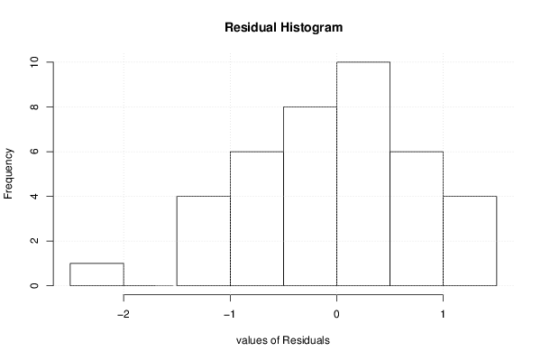
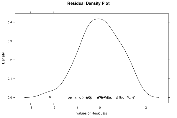
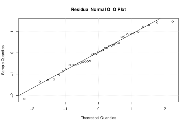
| Multiple Linear Regression - Residual Statistics | |
| Residual Standard Deviation | 0.905438 |
| Sum Squared Residuals | 27.054 |
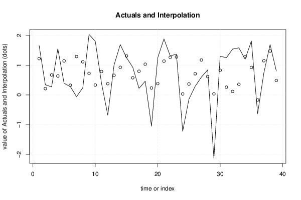
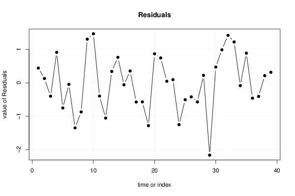
| Multiple Linear Regression - Actuals, Interpolation, and Residuals | |||
| Time or Index | Actuals | Interpolation Forecast | Residuals Prediction Error |
| 1 | 1.66 | 1.21862 | 0.441382 |
| 2 | 0.34 | 0.211054 | 0.128946 |
| 3 | 0.27 | 0.67106 | -0.40106 |
| 4 | 1.55 | 0.636254 | 0.913746 |
| 5 | 0.39 | 1.1422 | -0.752198 |
| 6 | 0.28 | 0.324875 | -0.0448753 |
| 7 | -0.06 | 1.28901 | -1.34901 |
| 8 | 0.24 | 1.11118 | -0.871185 |
| 9 | 2.03 | 0.722296 | 1.3077 |
| 10 | 1.8 | 0.331883 | 1.46812 |
| 11 | 0.39 | 0.78635 | -0.39635 |
| 12 | -0.68 | 0.375387 | -1.05539 |
| 13 | 1 | 0.659906 | 0.340094 |
| 14 | 1.69 | 0.926985 | 0.763015 |
| 15 | 1.25 | 1.31015 | -0.0601451 |
| 16 | 0.93 | 0.575386 | 0.354614 |
| 17 | 0.22 | 0.79525 | -0.57525 |
| 18 | 0.46 | 1.03037 | -0.570374 |
| 19 | -1.05 | 0.232636 | -1.28264 |
| 20 | 1.25 | 0.379924 | 0.870076 |
| 21 | 1.88 | 1.1346 | 0.745395 |
| 22 | 1.31 | 1.26304 | 0.0469649 |
| 23 | 1.37 | 1.27517 | 0.0948272 |
| 24 | -1.22 | 0.0322364 | -1.25224 |
| 25 | -0.14 | 0.365463 | -0.505463 |
| 26 | 0.29 | 0.710203 | -0.420203 |
| 27 | 0.6 | 1.17232 | -0.572317 |
| 28 | 0.84 | 0.615066 | 0.224934 |
| 29 | -2.13 | 0.0358327 | -2.16583 |
| 30 | 1.3 | 0.8272 | 0.4728 |
| 31 | 1.25 | 0.26071 | 0.98929 |
| 32 | 1.54 | 0.11702 | 1.42298 |
| 33 | 1.58 | 0.356427 | 1.22357 |
| 34 | 1.2 | 1.28392 | -0.083916 |
| 35 | 1.81 | 0.922407 | 0.887593 |
| 36 | -0.63 | -0.169667 | -0.460333 |
| 37 | 0.74 | 1.14713 | -0.407125 |
| 38 | 1.69 | 1.47539 | 0.214611 |
| 39 | 0.8 | 0.484768 | 0.315232 |
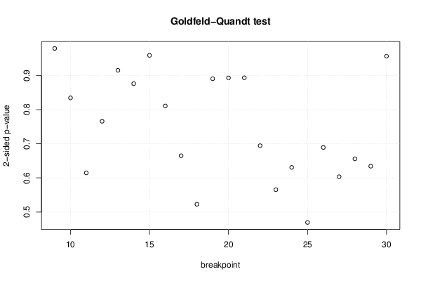
| Goldfeld-Quandt test for Heteroskedasticity | |||
| p-values | Alternative Hypothesis | ||
| breakpoint index | greater | 2-sided | less |
| 9 | 0.489607 | 0.979214 | 0.510393 |
| 10 | 0.417217 | 0.834435 | 0.582783 |
| 11 | 0.307266 | 0.614532 | 0.692734 |
| 12 | 0.382855 | 0.765711 | 0.617145 |
| 13 | 0.457571 | 0.915142 | 0.542429 |
| 14 | 0.561993 | 0.876015 | 0.438007 |
| 15 | 0.479456 | 0.958912 | 0.520544 |
| 16 | 0.405363 | 0.810726 | 0.594637 |
| 17 | 0.332385 | 0.66477 | 0.667615 |
| 18 | 0.261311 | 0.522622 | 0.738689 |
| 19 | 0.445234 | 0.890468 | 0.554766 |
| 20 | 0.446478 | 0.892955 | 0.553522 |
| 21 | 0.446639 | 0.893279 | 0.553361 |
| 22 | 0.347176 | 0.694352 | 0.652824 |
| 23 | 0.282644 | 0.565288 | 0.717356 |
| 24 | 0.315375 | 0.63075 | 0.684625 |
| 25 | 0.234672 | 0.469345 | 0.765328 |
| 26 | 0.344564 | 0.689129 | 0.655436 |
| 27 | 0.301599 | 0.603198 | 0.698401 |
| 28 | 0.327836 | 0.655672 | 0.672164 |
| 29 | 0.682901 | 0.634197 | 0.317099 |
| 30 | 0.521802 | 0.956397 | 0.478198 |
| Meta Analysis of Goldfeld-Quandt test for Heteroskedasticity | |||
| Description | # significant tests | % significant tests | OK/NOK |
| 1% type I error level | 0 | 0 | OK |
| 5% type I error level | 0 | 0 | OK |
| 10% type I error level | 0 | 0 | OK |