| Multiple Linear Regression - Estimated Regression Equation |
| HIV_Risk[t] = + 5.55387 + 0.0065663Per_Capita_Income[t] + 9.10475Prop_Population_on_Farms[t] + 0.24269Homicides[t] + e[t] |
| Warning: you did not specify the column number of the endogenous series! The first column was selected by default. |
| Multiple Linear Regression - Ordinary Least Squares | |||||
| Variable | Parameter | S.D. | T-STAT H0: parameter = 0 | 2-tail p-value | 1-tail p-value |
| (Intercept) | +5.554 | 7.898 | +7.0320e-01 | 0.4882 | 0.2441 |
| Per_Capita_Income | +0.006566 | 0.006239 | +1.0520e+00 | 0.3023 | 0.1511 |
| Prop_Population_on_Farms | +9.105 | 12.83 | +7.0970e-01 | 0.4842 | 0.2421 |
| Homicides | +0.2427 | 0.07284 | +3.3320e+00 | 0.002595 | 0.001297 |
| Multiple Linear Regression - Regression Statistics | |
| Multiple R | 0.6817 |
| R-squared | 0.4647 |
| Adjusted R-squared | 0.403 |
| F-TEST (value) | 7.525 |
| F-TEST (DF numerator) | 3 |
| F-TEST (DF denominator) | 26 |
| p-value | 0.0008779 |
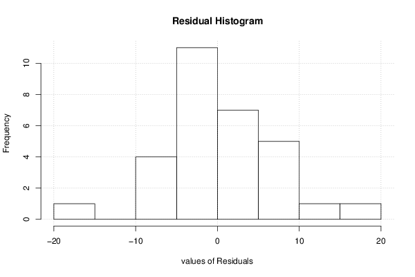
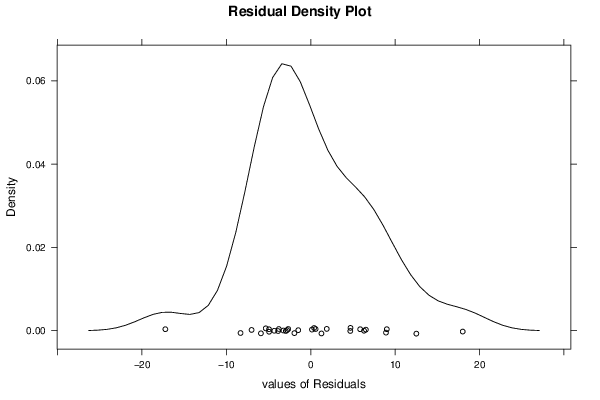
| Multiple Linear Regression - Residual Statistics | |
| Residual Standard Deviation | 7.4 |
| Sum Squared Residuals | 1424 |
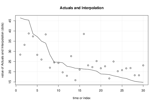
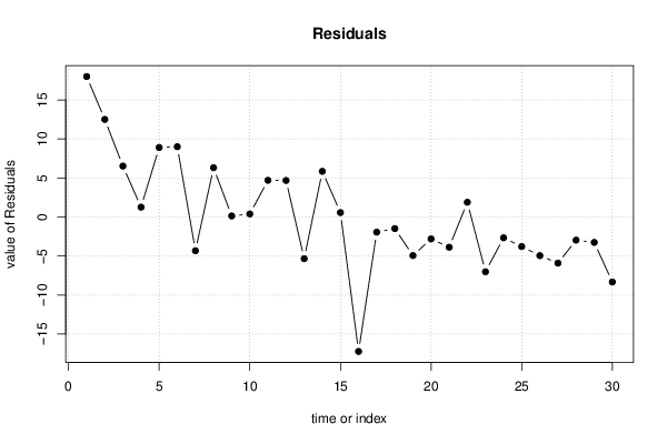
| Multiple Linear Regression - Actuals, Interpolation, and Residuals | |||
| Time or Index | Actuals | Interpolation Forecast | Residuals Prediction Error |
| 1 | 46.4 | 28.39 | 18.01 |
| 2 | 45.7 | 33.19 | 12.51 |
| 3 | 45.3 | 38.77 | 6.528 |
| 4 | 38.6 | 37.34 | 1.264 |
| 5 | 37.2 | 28.29 | 8.912 |
| 6 | 35 | 25.99 | 9.012 |
| 7 | 34 | 38.32 | -4.32 |
| 8 | 28.3 | 21.98 | 6.317 |
| 9 | 24.7 | 24.56 | 0.1387 |
| 10 | 24.7 | 24.31 | 0.3939 |
| 11 | 24.4 | 19.7 | 4.704 |
| 12 | 22.7 | 18.02 | 4.685 |
| 13 | 22.3 | 27.64 | -5.337 |
| 14 | 21.7 | 15.85 | 5.854 |
| 15 | 21.6 | 21.03 | 0.5697 |
| 16 | 21.3 | 38.53 | -17.23 |
| 17 | 21.2 | 23.14 | -1.939 |
| 18 | 20.8 | 22.28 | -1.481 |
| 19 | 20.3 | 25.24 | -4.938 |
| 20 | 18.9 | 21.7 | -2.805 |
| 21 | 18.8 | 22.67 | -3.872 |
| 22 | 18.6 | 16.71 | 1.893 |
| 23 | 18 | 25.01 | -7.015 |
| 24 | 17.6 | 20.27 | -2.665 |
| 25 | 17 | 20.79 | -3.789 |
| 26 | 16.7 | 21.65 | -4.949 |
| 27 | 15.9 | 21.81 | -5.908 |
| 28 | 15.3 | 18.26 | -2.96 |
| 29 | 15 | 18.25 | -3.253 |
| 30 | 14.8 | 23.12 | -8.324 |
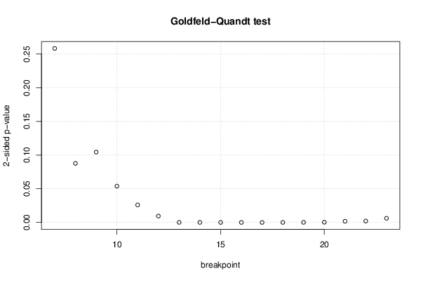
| Goldfeld-Quandt test for Heteroskedasticity | |||
| p-values | Alternative Hypothesis | ||
| breakpoint index | greater | 2-sided | less |
| 7 | 0.8709 | 0.2583 | 0.1291 |
| 8 | 0.9562 | 0.08767 | 0.04384 |
| 9 | 0.9478 | 0.1044 | 0.05222 |
| 10 | 0.973 | 0.05398 | 0.02699 |
| 11 | 0.987 | 0.026 | 0.013 |
| 12 | 0.9953 | 0.009465 | 0.004732 |
| 13 | 0.9999 | 0.0001367 | 6.836e-05 |
| 14 | 1 | 5.608e-05 | 2.804e-05 |
| 15 | 1 | 3.137e-05 | 1.568e-05 |
| 16 | 1 | 7.154e-06 | 3.577e-06 |
| 17 | 1 | 1.759e-05 | 8.796e-06 |
| 18 | 1 | 4.844e-05 | 2.422e-05 |
| 19 | 0.9999 | 0.0001214 | 6.071e-05 |
| 20 | 0.9998 | 0.0003135 | 0.0001567 |
| 21 | 0.9991 | 0.001808 | 0.0009038 |
| 22 | 0.999 | 0.002041 | 0.001021 |
| 23 | 0.9969 | 0.006171 | 0.003086 |
| Meta Analysis of Goldfeld-Quandt test for Heteroskedasticity | |||
| Description | # significant tests | % significant tests | OK/NOK |
| 1% type I error level | 12 | 0.7059 | NOK |
| 5% type I error level | 13 | 0.764706 | NOK |
| 10% type I error level | 15 | 0.882353 | NOK |