| Multiple Linear Regression - Estimated Regression Equation |
| a[t] = -44.9882 + 1.7506b[t] + 0.367952c[t] + e[t] |
| Multiple Linear Regression - Ordinary Least Squares | |||||
| Variable | Parameter | S.D. | T-STAT H0: parameter = 0 | 2-tail p-value | 1-tail p-value |
| (Intercept) | -44.99 | 6.553 | -6.8660e+00 | 2.241e-07 | 1.12e-07 |
| b | +1.751 | 0.08576 | +2.0410e+01 | 6.058e-18 | 3.029e-18 |
| c | +0.3679 | 0.128 | +2.8730e+00 | 0.007818 | 0.003909 |
| Multiple Linear Regression - Regression Statistics | |
| Multiple R | 0.9711 |
| R-squared | 0.943 |
| Adjusted R-squared | 0.9388 |
| F-TEST (value) | 223.5 |
| F-TEST (DF numerator) | 2 |
| F-TEST (DF denominator) | 27 |
| p-value | 0 |
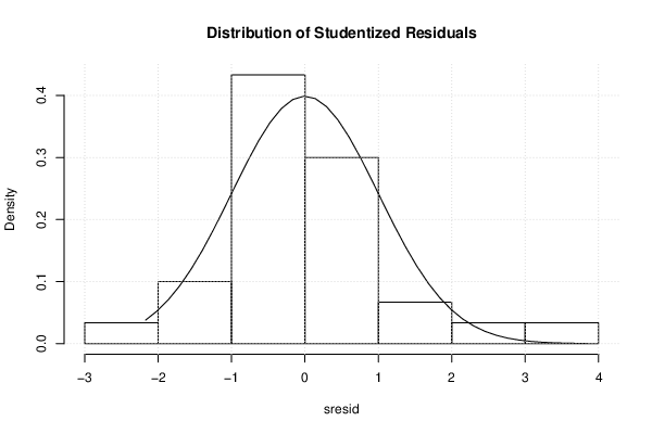
| Multiple Linear Regression - Residual Statistics | |
| Residual Standard Deviation | 3.097 |
| Sum Squared Residuals | 258.9 |
| Menu of Residual Diagnostics | |
| Description | Link |
| Histogram | Compute |
| Central Tendency | Compute |
| QQ Plot | Compute |
| Kernel Density Plot | Compute |
| Skewness/Kurtosis Test | Compute |
| Skewness-Kurtosis Plot | Compute |
| Harrell-Davis Plot | Compute |
| Bootstrap Plot -- Central Tendency | Compute |
| Blocked Bootstrap Plot -- Central Tendency | Compute |
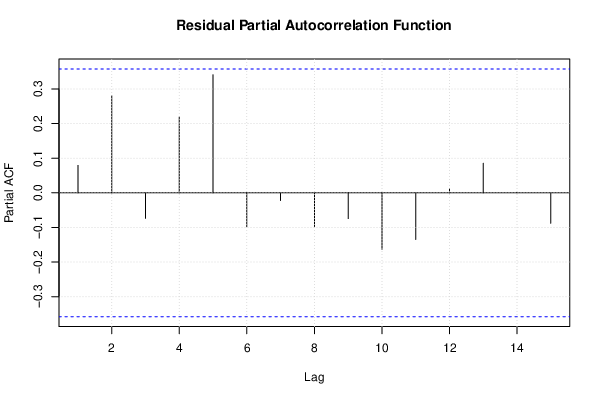
| (Partial) Autocorrelation Plot | Compute |
| Spectral Analysis | Compute |
| Tukey lambda PPCC Plot | Compute |
| Box-Cox Normality Plot | Compute |
| Summary Statistics | Compute |
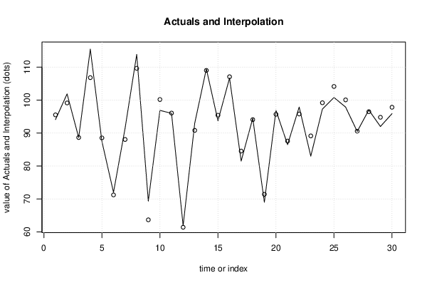
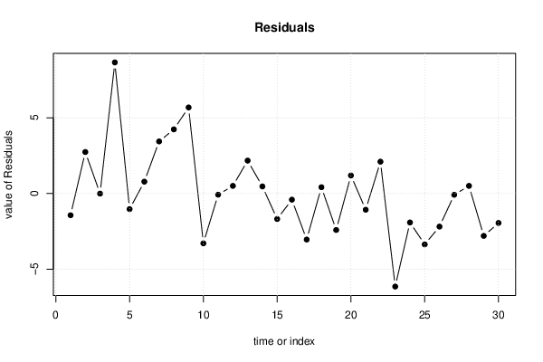
| Multiple Linear Regression - Actuals, Interpolation, and Residuals | |||
| Time or Index | Actuals | Interpolation Forecast | Residuals Prediction Error |
| 1 | 94.1 | 95.54 | -1.436 |
| 2 | 101.9 | 99.16 | 2.741 |
| 3 | 88.65 | 88.66 | -0.006204 |
| 4 | 115.5 | 106.8 | 8.658 |
| 5 | 87.5 | 88.53 | -1.032 |
| 6 | 72 | 71.22 | 0.7821 |
| 7 | 91.5 | 88.06 | 3.437 |
| 8 | 113.9 | 109.7 | 4.236 |
| 9 | 69.34 | 63.66 | 5.684 |
| 10 | 96.9 | 100.2 | -3.291 |
| 11 | 96 | 96.08 | -0.07745 |
| 12 | 61.9 | 61.4 | 0.5029 |
| 13 | 93 | 90.83 | 2.173 |
| 14 | 109.5 | 109 | 0.4671 |
| 15 | 93.75 | 95.43 | -1.683 |
| 16 | 106.7 | 107.1 | -0.4079 |
| 17 | 81.5 | 84.54 | -3.04 |
| 18 | 94.5 | 94.08 | 0.416 |
| 19 | 69 | 71.41 | -2.41 |
| 20 | 96.9 | 95.71 | 1.191 |
| 21 | 86.5 | 87.57 | -1.072 |
| 22 | 97.9 | 95.8 | 2.101 |
| 23 | 83 | 89.15 | -6.146 |
| 24 | 97.3 | 99.21 | -1.913 |
| 25 | 100.8 | 104.2 | -3.364 |
| 26 | 97.9 | 100.1 | -2.186 |
| 27 | 90.5 | 90.58 | -0.08219 |
| 28 | 97 | 96.5 | 0.5034 |
| 29 | 92 | 94.8 | -2.8 |
| 30 | 95.9 | 97.85 | -1.947 |
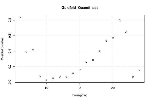
| Goldfeld-Quandt test for Heteroskedasticity | |||
| p-values | Alternative Hypothesis | ||
| breakpoint index | greater | 2-sided | less |
| 6 | 0.582 | 0.836 | 0.418 |
| 7 | 0.8032 | 0.3937 | 0.1968 |
| 8 | 0.7906 | 0.4189 | 0.2094 |
| 9 | 0.9636 | 0.07286 | 0.03643 |
| 10 | 0.9862 | 0.02751 | 0.01375 |
| 11 | 0.9758 | 0.04839 | 0.02419 |
| 12 | 0.9653 | 0.06936 | 0.03468 |
| 13 | 0.9663 | 0.06732 | 0.03366 |
| 14 | 0.9436 | 0.1128 | 0.05639 |
| 15 | 0.9186 | 0.1629 | 0.08144 |
| 16 | 0.8693 | 0.2614 | 0.1307 |
| 17 | 0.8572 | 0.2857 | 0.1428 |
| 18 | 0.7987 | 0.4026 | 0.2013 |
| 19 | 0.734 | 0.532 | 0.266 |
| 20 | 0.7138 | 0.5724 | 0.2862 |
| 21 | 0.6008 | 0.7983 | 0.3992 |
| 22 | 0.6782 | 0.6435 | 0.3218 |
| 23 | 0.9658 | 0.06841 | 0.03421 |
| 24 | 0.9202 | 0.1596 | 0.0798 |
| Meta Analysis of Goldfeld-Quandt test for Heteroskedasticity | |||
| Description | # significant tests | % significant tests | OK/NOK |
| 1% type I error level | 0 | 0 | OK |
| 5% type I error level | 2 | 0.105263 | NOK |
| 10% type I error level | 6 | 0.315789 | NOK |
| Ramsey RESET F-Test for powers (2 and 3) of fitted values |
> reset_test_fitted RESET test data: mylm RESET = 2.7863, df1 = 2, df2 = 25, p-value = 0.08083 |
| Ramsey RESET F-Test for powers (2 and 3) of regressors |
> reset_test_regressors RESET test data: mylm RESET = 1.9404, df1 = 4, df2 = 23, p-value = 0.1377 |
| Ramsey RESET F-Test for powers (2 and 3) of principal components |
> reset_test_principal_components RESET test data: mylm RESET = 3.0801, df1 = 2, df2 = 25, p-value = 0.06371 |
| Variance Inflation Factors (Multicollinearity) |
> vif
       b        c
1.016201 1.016201
|