| Multiple Linear Regression - Estimated Regression Equation |
| BCTsRes[t] = + 98.4748 -0.5105Cito[t] + 0.0795Lot[t] + 0.239076CD[t] + e[t] |
| Multiple Linear Regression - Ordinary Least Squares | |||||
| Variable | Parameter | S.D. | T-STAT H0: parameter = 0 | 2-tail p-value | 1-tail p-value |
| (Intercept) | +98.47 | 0.6505 | +1.5140e+02 | 4.368e-52 | 2.184e-52 |
| Cito | -0.5105 | 0.2733 | -1.8680e+00 | 0.06991 | 0.03496 |
| Lot | +0.0795 | 0.2733 | +2.9090e-01 | 0.7728 | 0.3864 |
| CD | +0.2391 | 0.04757 | +5.0260e+00 | 1.389e-05 | 6.947e-06 |
| Multiple Linear Regression - Regression Statistics | |
| Multiple R | 0.6669 |
| R-squared | 0.4447 |
| Adjusted R-squared | 0.3984 |
| F-TEST (value) | 9.61 |
| F-TEST (DF numerator) | 3 |
| F-TEST (DF denominator) | 36 |
| p-value | 8.473e-05 |
| Multiple Linear Regression - Residual Statistics | |
| Residual Standard Deviation | 0.8642 |
| Sum Squared Residuals | 26.89 |
| Menu of Residual Diagnostics | |
| Description | Link |
| Histogram | Compute |
| Central Tendency | Compute |
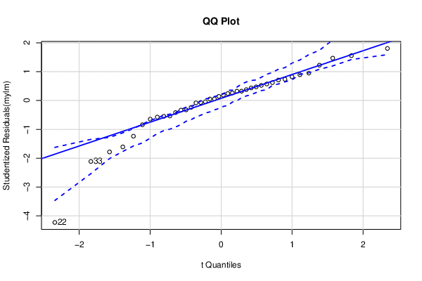
| QQ Plot | Compute |
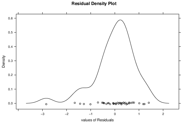
| Kernel Density Plot | Compute |
| Skewness/Kurtosis Test | Compute |
| Skewness-Kurtosis Plot | Compute |
| Harrell-Davis Plot | Compute |
| Bootstrap Plot -- Central Tendency | Compute |
| Blocked Bootstrap Plot -- Central Tendency | Compute |
| (Partial) Autocorrelation Plot | Compute |
| Spectral Analysis | Compute |
| Tukey lambda PPCC Plot | Compute |
| Box-Cox Normality Plot | Compute |
| Summary Statistics | Compute |
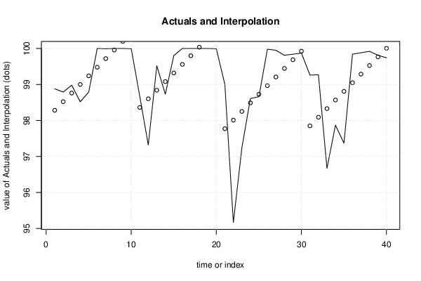
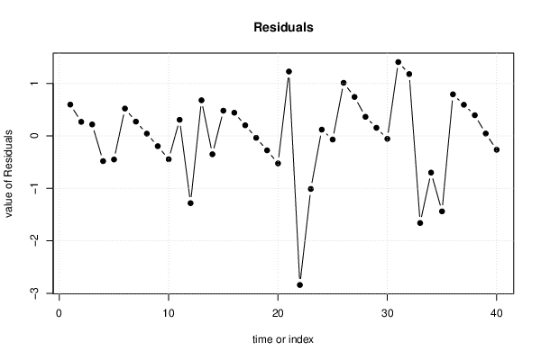
| Multiple Linear Regression - Actuals, Interpolation, and Residuals | |||
| Time or Index | Actuals | Interpolation Forecast | Residuals Prediction Error |
| 1 | 98.88 | 98.28 | 0.5971 |
| 2 | 98.79 | 98.52 | 0.268 |
| 3 | 98.98 | 98.76 | 0.2189 |
| 4 | 98.52 | 99 | -0.4801 |
| 5 | 98.79 | 99.24 | -0.4492 |
| 6 | 100 | 99.48 | 0.5217 |
| 7 | 99.99 | 99.72 | 0.2726 |
| 8 | 100 | 99.96 | 0.04356 |
| 9 | 100 | 100.2 | -0.1955 |
| 10 | 99.99 | 100.4 | -0.4446 |
| 11 | 98.67 | 98.36 | 0.3076 |
| 12 | 97.32 | 98.6 | -1.281 |
| 13 | 99.52 | 98.84 | 0.6794 |
| 14 | 98.73 | 99.08 | -0.3496 |
| 15 | 99.8 | 99.32 | 0.4813 |
| 16 | 100 | 99.56 | 0.4422 |
| 17 | 100 | 99.8 | 0.2031 |
| 18 | 100 | 100 | -0.03594 |
| 19 | 100 | 100.3 | -0.275 |
| 20 | 99.99 | 100.5 | -0.5241 |
| 21 | 99 | 97.77 | 1.228 |
| 22 | 95.17 | 98.01 | -2.841 |
| 23 | 97.24 | 98.25 | -1.011 |
| 24 | 98.61 | 98.49 | 0.1204 |
| 25 | 98.66 | 98.73 | -0.06871 |
| 26 | 99.98 | 98.97 | 1.012 |
| 27 | 99.95 | 99.21 | 0.7431 |
| 28 | 99.81 | 99.45 | 0.3641 |
| 29 | 99.84 | 99.69 | 0.155 |
| 30 | 99.87 | 99.92 | -0.05409 |
| 31 | 99.26 | 97.85 | 1.408 |
| 32 | 99.27 | 98.09 | 1.179 |
| 33 | 96.67 | 98.33 | -1.66 |
| 34 | 97.87 | 98.57 | -0.6991 |
| 35 | 97.37 | 98.81 | -1.438 |
| 36 | 99.84 | 99.05 | 0.7927 |
| 37 | 99.88 | 99.29 | 0.5936 |
| 38 | 99.92 | 99.53 | 0.3946 |
| 39 | 99.81 | 99.76 | 0.04548 |
| 40 | 99.74 | 100 | -0.2636 |
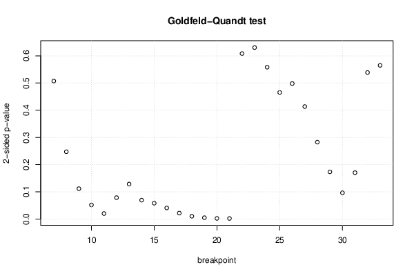
| Goldfeld-Quandt test for Heteroskedasticity | |||
| p-values | Alternative Hypothesis | ||
| breakpoint index | greater | 2-sided | less |
| 7 | 0.2536 | 0.5071 | 0.7464 |
| 8 | 0.1237 | 0.2475 | 0.8763 |
| 9 | 0.05585 | 0.1117 | 0.9442 |
| 10 | 0.02599 | 0.05198 | 0.974 |
| 11 | 0.01012 | 0.02025 | 0.9899 |
| 12 | 0.03936 | 0.07872 | 0.9606 |
| 13 | 0.06425 | 0.1285 | 0.9358 |
| 14 | 0.03475 | 0.06949 | 0.9653 |
| 15 | 0.02916 | 0.05833 | 0.9708 |
| 16 | 0.0204 | 0.0408 | 0.9796 |
| 17 | 0.01095 | 0.02189 | 0.9891 |
| 18 | 0.005221 | 0.01044 | 0.9948 |
| 19 | 0.002447 | 0.004893 | 0.9976 |
| 20 | 0.001208 | 0.002416 | 0.9988 |
| 21 | 0.001043 | 0.002086 | 0.999 |
| 22 | 0.3041 | 0.6082 | 0.6959 |
| 23 | 0.3151 | 0.6302 | 0.6849 |
| 24 | 0.2791 | 0.5581 | 0.7209 |
| 25 | 0.2326 | 0.4653 | 0.7674 |
| 26 | 0.249 | 0.498 | 0.751 |
| 27 | 0.2067 | 0.4134 | 0.7933 |
| 28 | 0.1413 | 0.2827 | 0.8587 |
| 29 | 0.08672 | 0.1734 | 0.9133 |
| 30 | 0.04822 | 0.09644 | 0.9518 |
| 31 | 0.08524 | 0.1705 | 0.9148 |
| 32 | 0.2693 | 0.5386 | 0.7307 |
| 33 | 0.2824 | 0.5649 | 0.7176 |
| Meta Analysis of Goldfeld-Quandt test for Heteroskedasticity | |||
| Description | # significant tests | % significant tests | OK/NOK |
| 1% type I error level | 3 | 0.1111 | NOK |
| 5% type I error level | 7 | 0.259259 | NOK |
| 10% type I error level | 12 | 0.444444 | NOK |
| Ramsey RESET F-Test for powers (2 and 3) of fitted values |
> reset_test_fitted RESET test data: mylm RESET = 2.9896, df1 = 2, df2 = 34, p-value = 0.06367 |
| Ramsey RESET F-Test for powers (2 and 3) of regressors |
> reset_test_regressors RESET test data: mylm RESET = 1.6308, df1 = 6, df2 = 30, p-value = 0.1731 |
| Ramsey RESET F-Test for powers (2 and 3) of principal components |
> reset_test_principal_components RESET test data: mylm RESET = 5.5448, df1 = 2, df2 = 34, p-value = 0.008239 |
| Variance Inflation Factors (Multicollinearity) |
> vif Cito Lot CD 1 1 1 |