Free Statistics

of Irreproducible Research!

Author's title

Author*Unverified author*
R Software Modulerwasp_boxcoxnorm.wasp
Title produced by softwareBox-Cox Normality Plot
Date of computationMon, 10 Aug 2020 18:26:18 +0200
Cite this page as followsStatistical Computations at FreeStatistics.org, Office for Research Development and Education, URL https://freestatistics.org/blog/index.php?v=date/2020/Aug/10/t1597079059e3srnmkg0fs7dsq.htm/, Retrieved Sat, 20 Apr 2024 13:58:10 +0000
Statistical Computations at FreeStatistics.org, Office for Research Development and Education, URL https://freestatistics.org/blog/index.php?pk=319215, Retrieved Sat, 20 Apr 2024 13:58:10 +0000
QR Codes:

Original text written by user:
IsPrivate?No (this computation is public)
User-defined keywords
Estimated Impact113
Family? (F = Feedback message, R = changed R code, M = changed R Module, P = changed Parameters, D = changed Data)
-       [Box-Cox Normality Plot] [Box Cox] [2020-08-10 16:26:18] [d41d8cd98f00b204e9800998ecf8427e] [Current]
Feedback Forum

Post a new message
Dataseries X:
12
14
56
20
15
16
17.5
18
19
20
15
16
17
18
19
20
15
16
17
14
16
18.5
19.5
15.5
16.5
17
18.5
19.5
22
42
32
34
32
26
38
36
24.6
35
35
21
29
18
22
34
21
38
36
32
21
28.5


Summary of computational transaction
Raw Input view raw input (R code)
Raw Outputview raw output of R engine
Computing time2 seconds
R ServerBig Analytics Cloud Computing Center

\begin{tabular}{lllllllll}
\hline
Summary of computational transaction \tabularnewline
Raw Input view raw input (R code)  \tabularnewline
Raw Outputview raw output of R engine  \tabularnewline
Computing time2 seconds \tabularnewline
R ServerBig Analytics Cloud Computing Center \tabularnewline
\hline
\end{tabular}
%Source: https://freestatistics.org/blog/index.php?pk=319215&T=0

[TABLE]
[ROW]
Summary of computational transaction[/C][/ROW] [ROW]Raw Input[/C] view raw input (R code) [/C][/ROW] [ROW]Raw Output[/C]view raw output of R engine [/C][/ROW] [ROW]Computing time[/C]2 seconds[/C][/ROW] [ROW]R Server[/C]Big Analytics Cloud Computing Center[/C][/ROW] [/TABLE] Source: https://freestatistics.org/blog/index.php?pk=319215&T=0

Globally Unique Identifier (entire table): ba.freestatistics.org/blog/index.php?pk=319215&T=0

As an alternative you can also use a QR Code:  

The GUIDs for individual cells are displayed in the table below:

Summary of computational transaction
Raw Input view raw input (R code)
Raw Outputview raw output of R engine
Computing time2 seconds
R ServerBig Analytics Cloud Computing Center


Box-Cox Normality Plot
# observations x50
maximum correlation0.98115347693728
optimal lambda-1.25
transformation formulafor all lambda <> 0 : T(Y) = (Y^lambda - 1) / lambda

\begin{tabular}{lllllllll}
\hline
Box-Cox Normality Plot \tabularnewline
# observations x & 50 \tabularnewline
maximum correlation & 0.98115347693728 \tabularnewline
optimal lambda & -1.25 \tabularnewline
transformation formula & for all lambda <> 0 : T(Y) = (Y^lambda - 1) / lambda \tabularnewline
\hline
\end{tabular}
%Source: https://freestatistics.org/blog/index.php?pk=319215&T=1

[TABLE]
[ROW][C]Box-Cox Normality Plot[/C][/ROW]
[ROW][C]# observations x[/C][C]50[/C][/ROW]
[ROW][C]maximum correlation[/C][C]0.98115347693728[/C][/ROW]
[ROW][C]optimal lambda[/C][C]-1.25[/C][/ROW]
[ROW][C]transformation formula[/C][C]for all lambda <> 0 : T(Y) = (Y^lambda - 1) / lambda[/C][/ROW]
[/TABLE]
Source: https://freestatistics.org/blog/index.php?pk=319215&T=1

Globally Unique Identifier (entire table): ba.freestatistics.org/blog/index.php?pk=319215&T=1

As an alternative you can also use a QR Code:  

The GUIDs for individual cells are displayed in the table below:

Box-Cox Normality Plot
# observations x50
maximum correlation0.98115347693728
optimal lambda-1.25
transformation formulafor all lambda <> 0 : T(Y) = (Y^lambda - 1) / lambda


Obs.OriginalTransformed
1120.764181002272549
2140.770458676916733
3560.79477778253065
4200.781085167819936
5150.772899586765087
6160.775
717.50.777649233260119
8180.778422587924119
9190.779832689455007
10200.781085167819936
11150.772899586765087
12160.775
13170.776824514799743
14180.778422587924119
15190.779832689455007
16200.781085167819936
17150.772899586765087
18160.775
19170.776824514799743
20140.770458676916733
21160.775
2218.50.779149074983456
2319.50.780476992424974
2415.50.773987903033469
2516.50.775943355149865
26170.776824514799743
2718.50.779149074983456
2819.50.780476992424974
29220.783209577056578
30420.792517816173324
31320.789488794809329
32340.790255908786669
33320.789488794809329
34260.786373845714796
35380.791520690428704
36360.79092781576747
3724.60.785397705498621
38350.790602660185131
39350.790602660185131
40210.782204267515116
41290.788112446359754
42180.778422587924119
43220.783209577056578
44340.790255908786669
45210.782204267515116
46380.791520690428704
47360.79092781576747
48320.789488794809329
49210.782204267515116
5028.50.787851185189415

\begin{tabular}{lllllllll}
\hline
Obs. & Original & Transformed \tabularnewline
1 & 12 & 0.764181002272549 \tabularnewline
2 & 14 & 0.770458676916733 \tabularnewline
3 & 56 & 0.79477778253065 \tabularnewline
4 & 20 & 0.781085167819936 \tabularnewline
5 & 15 & 0.772899586765087 \tabularnewline
6 & 16 & 0.775 \tabularnewline
7 & 17.5 & 0.777649233260119 \tabularnewline
8 & 18 & 0.778422587924119 \tabularnewline
9 & 19 & 0.779832689455007 \tabularnewline
10 & 20 & 0.781085167819936 \tabularnewline
11 & 15 & 0.772899586765087 \tabularnewline
12 & 16 & 0.775 \tabularnewline
13 & 17 & 0.776824514799743 \tabularnewline
14 & 18 & 0.778422587924119 \tabularnewline
15 & 19 & 0.779832689455007 \tabularnewline
16 & 20 & 0.781085167819936 \tabularnewline
17 & 15 & 0.772899586765087 \tabularnewline
18 & 16 & 0.775 \tabularnewline
19 & 17 & 0.776824514799743 \tabularnewline
20 & 14 & 0.770458676916733 \tabularnewline
21 & 16 & 0.775 \tabularnewline
22 & 18.5 & 0.779149074983456 \tabularnewline
23 & 19.5 & 0.780476992424974 \tabularnewline
24 & 15.5 & 0.773987903033469 \tabularnewline
25 & 16.5 & 0.775943355149865 \tabularnewline
26 & 17 & 0.776824514799743 \tabularnewline
27 & 18.5 & 0.779149074983456 \tabularnewline
28 & 19.5 & 0.780476992424974 \tabularnewline
29 & 22 & 0.783209577056578 \tabularnewline
30 & 42 & 0.792517816173324 \tabularnewline
31 & 32 & 0.789488794809329 \tabularnewline
32 & 34 & 0.790255908786669 \tabularnewline
33 & 32 & 0.789488794809329 \tabularnewline
34 & 26 & 0.786373845714796 \tabularnewline
35 & 38 & 0.791520690428704 \tabularnewline
36 & 36 & 0.79092781576747 \tabularnewline
37 & 24.6 & 0.785397705498621 \tabularnewline
38 & 35 & 0.790602660185131 \tabularnewline
39 & 35 & 0.790602660185131 \tabularnewline
40 & 21 & 0.782204267515116 \tabularnewline
41 & 29 & 0.788112446359754 \tabularnewline
42 & 18 & 0.778422587924119 \tabularnewline
43 & 22 & 0.783209577056578 \tabularnewline
44 & 34 & 0.790255908786669 \tabularnewline
45 & 21 & 0.782204267515116 \tabularnewline
46 & 38 & 0.791520690428704 \tabularnewline
47 & 36 & 0.79092781576747 \tabularnewline
48 & 32 & 0.789488794809329 \tabularnewline
49 & 21 & 0.782204267515116 \tabularnewline
50 & 28.5 & 0.787851185189415 \tabularnewline
\hline
\end{tabular}
%Source: https://freestatistics.org/blog/index.php?pk=319215&T=2

[TABLE]
[ROW][C]Obs.[/C][C]Original[/C][C]Transformed[/C][/ROW]
[ROW][C]1[/C][C]12[/C][C]0.764181002272549[/C][/ROW]
[ROW][C]2[/C][C]14[/C][C]0.770458676916733[/C][/ROW]
[ROW][C]3[/C][C]56[/C][C]0.79477778253065[/C][/ROW]
[ROW][C]4[/C][C]20[/C][C]0.781085167819936[/C][/ROW]
[ROW][C]5[/C][C]15[/C][C]0.772899586765087[/C][/ROW]
[ROW][C]6[/C][C]16[/C][C]0.775[/C][/ROW]
[ROW][C]7[/C][C]17.5[/C][C]0.777649233260119[/C][/ROW]
[ROW][C]8[/C][C]18[/C][C]0.778422587924119[/C][/ROW]
[ROW][C]9[/C][C]19[/C][C]0.779832689455007[/C][/ROW]
[ROW][C]10[/C][C]20[/C][C]0.781085167819936[/C][/ROW]
[ROW][C]11[/C][C]15[/C][C]0.772899586765087[/C][/ROW]
[ROW][C]12[/C][C]16[/C][C]0.775[/C][/ROW]
[ROW][C]13[/C][C]17[/C][C]0.776824514799743[/C][/ROW]
[ROW][C]14[/C][C]18[/C][C]0.778422587924119[/C][/ROW]
[ROW][C]15[/C][C]19[/C][C]0.779832689455007[/C][/ROW]
[ROW][C]16[/C][C]20[/C][C]0.781085167819936[/C][/ROW]
[ROW][C]17[/C][C]15[/C][C]0.772899586765087[/C][/ROW]
[ROW][C]18[/C][C]16[/C][C]0.775[/C][/ROW]
[ROW][C]19[/C][C]17[/C][C]0.776824514799743[/C][/ROW]
[ROW][C]20[/C][C]14[/C][C]0.770458676916733[/C][/ROW]
[ROW][C]21[/C][C]16[/C][C]0.775[/C][/ROW]
[ROW][C]22[/C][C]18.5[/C][C]0.779149074983456[/C][/ROW]
[ROW][C]23[/C][C]19.5[/C][C]0.780476992424974[/C][/ROW]
[ROW][C]24[/C][C]15.5[/C][C]0.773987903033469[/C][/ROW]
[ROW][C]25[/C][C]16.5[/C][C]0.775943355149865[/C][/ROW]
[ROW][C]26[/C][C]17[/C][C]0.776824514799743[/C][/ROW]
[ROW][C]27[/C][C]18.5[/C][C]0.779149074983456[/C][/ROW]
[ROW][C]28[/C][C]19.5[/C][C]0.780476992424974[/C][/ROW]
[ROW][C]29[/C][C]22[/C][C]0.783209577056578[/C][/ROW]
[ROW][C]30[/C][C]42[/C][C]0.792517816173324[/C][/ROW]
[ROW][C]31[/C][C]32[/C][C]0.789488794809329[/C][/ROW]
[ROW][C]32[/C][C]34[/C][C]0.790255908786669[/C][/ROW]
[ROW][C]33[/C][C]32[/C][C]0.789488794809329[/C][/ROW]
[ROW][C]34[/C][C]26[/C][C]0.786373845714796[/C][/ROW]
[ROW][C]35[/C][C]38[/C][C]0.791520690428704[/C][/ROW]
[ROW][C]36[/C][C]36[/C][C]0.79092781576747[/C][/ROW]
[ROW][C]37[/C][C]24.6[/C][C]0.785397705498621[/C][/ROW]
[ROW][C]38[/C][C]35[/C][C]0.790602660185131[/C][/ROW]
[ROW][C]39[/C][C]35[/C][C]0.790602660185131[/C][/ROW]
[ROW][C]40[/C][C]21[/C][C]0.782204267515116[/C][/ROW]
[ROW][C]41[/C][C]29[/C][C]0.788112446359754[/C][/ROW]
[ROW][C]42[/C][C]18[/C][C]0.778422587924119[/C][/ROW]
[ROW][C]43[/C][C]22[/C][C]0.783209577056578[/C][/ROW]
[ROW][C]44[/C][C]34[/C][C]0.790255908786669[/C][/ROW]
[ROW][C]45[/C][C]21[/C][C]0.782204267515116[/C][/ROW]
[ROW][C]46[/C][C]38[/C][C]0.791520690428704[/C][/ROW]
[ROW][C]47[/C][C]36[/C][C]0.79092781576747[/C][/ROW]
[ROW][C]48[/C][C]32[/C][C]0.789488794809329[/C][/ROW]
[ROW][C]49[/C][C]21[/C][C]0.782204267515116[/C][/ROW]
[ROW][C]50[/C][C]28.5[/C][C]0.787851185189415[/C][/ROW]
[/TABLE]
Source: https://freestatistics.org/blog/index.php?pk=319215&T=2

Globally Unique Identifier (entire table): ba.freestatistics.org/blog/index.php?pk=319215&T=2

As an alternative you can also use a QR Code:  

The GUIDs for individual cells are displayed in the table below:

Obs.OriginalTransformed
1120.764181002272549
2140.770458676916733
3560.79477778253065
4200.781085167819936
5150.772899586765087
6160.775
717.50.777649233260119
8180.778422587924119
9190.779832689455007
10200.781085167819936
11150.772899586765087
12160.775
13170.776824514799743
14180.778422587924119
15190.779832689455007
16200.781085167819936
17150.772899586765087
18160.775
19170.776824514799743
20140.770458676916733
21160.775
2218.50.779149074983456
2319.50.780476992424974
2415.50.773987903033469
2516.50.775943355149865
26170.776824514799743
2718.50.779149074983456
2819.50.780476992424974
29220.783209577056578
30420.792517816173324
31320.789488794809329
32340.790255908786669
33320.789488794809329
34260.786373845714796
35380.791520690428704
36360.79092781576747
3724.60.785397705498621
38350.790602660185131
39350.790602660185131
40210.782204267515116
41290.788112446359754
42180.778422587924119
43220.783209577056578
44340.790255908786669
45210.782204267515116
46380.791520690428704
47360.79092781576747
48320.789488794809329
49210.782204267515116
5028.50.787851185189415


Maximum Likelihood Estimation of Lambda
> summary(mypT)
bcPower Transformation to Normality 
  Est Power Rounded Pwr Wald Lwr Bnd Wald Upr Bnd
x   -0.9778          -1      -1.8204      -0.1353
Likelihood ratio test that transformation parameter is equal to 0
 (log transformation)
                           LRT df     pval
LR test, lambda = (0) 5.342812  1 0.020808
Likelihood ratio test that no transformation is needed
                           LRT df       pval
LR test, lambda = (1) 22.68833  1 1.9052e-06

\begin{tabular}{lllllllll}
\hline
Maximum Likelihood Estimation of Lambda \tabularnewline
> summary(mypT)
bcPower Transformation to Normality 
  Est Power Rounded Pwr Wald Lwr Bnd Wald Upr Bnd
x   -0.9778          -1      -1.8204      -0.1353
Likelihood ratio test that transformation parameter is equal to 0
 (log transformation)
                           LRT df     pval
LR test, lambda = (0) 5.342812  1 0.020808
Likelihood ratio test that no transformation is needed
                           LRT df       pval
LR test, lambda = (1) 22.68833  1 1.9052e-06
\tabularnewline \hline \end{tabular} %Source: https://freestatistics.org/blog/index.php?pk=319215&T=3

[TABLE]
[ROW][C]Maximum Likelihood Estimation of Lambda[/C][/ROW]
[ROW][C]
> summary(mypT)
bcPower Transformation to Normality 
  Est Power Rounded Pwr Wald Lwr Bnd Wald Upr Bnd
x   -0.9778          -1      -1.8204      -0.1353
Likelihood ratio test that transformation parameter is equal to 0
 (log transformation)
                           LRT df     pval
LR test, lambda = (0) 5.342812  1 0.020808
Likelihood ratio test that no transformation is needed
                           LRT df       pval
LR test, lambda = (1) 22.68833  1 1.9052e-06
[/C][/ROW] [/TABLE] Source: https://freestatistics.org/blog/index.php?pk=319215&T=3

Globally Unique Identifier (entire table): ba.freestatistics.org/blog/index.php?pk=319215&T=3

As an alternative you can also use a QR Code:  

The GUIDs for individual cells are displayed in the table below:

Maximum Likelihood Estimation of Lambda
> summary(mypT)
bcPower Transformation to Normality 
  Est Power Rounded Pwr Wald Lwr Bnd Wald Upr Bnd
x   -0.9778          -1      -1.8204      -0.1353
Likelihood ratio test that transformation parameter is equal to 0
 (log transformation)
                           LRT df     pval
LR test, lambda = (0) 5.342812  1 0.020808
Likelihood ratio test that no transformation is needed
                           LRT df       pval
LR test, lambda = (1) 22.68833  1 1.9052e-06


Parameters (Session):
par1 = Full Box-Cox transform ; par2 = -2 ; par3 = 2 ; par4 = 0 ; par5 = Yes ;
Parameters (R input):
par1 = Full Box-Cox transform ; par2 = -2 ; par3 = 2 ; par4 = 0 ; par5 = Yes ;
R code (references can be found in the software module):
par5 <- 'Yes'
par4 <- '0'
par3 <- '2'
par2 <- '-2'
par1 <- 'Full Box-Cox transform'
library(car)
par2 <- abs(as.numeric(par2)*100)
par3 <- as.numeric(par3)*100
if(par4=='') par4 <- 0
par4 <- as.numeric(par4)
numlam <- par2 + par3 + 1
x <- x + par4
n <- length(x)
c <- array(NA,dim=c(numlam))
l <- array(NA,dim=c(numlam))
mx <- -1
mxli <- -999
for (i in 1:numlam)
{
l[i] <- (i-par2-1)/100
if (l[i] != 0)
{
if (par1 == 'Full Box-Cox transform') x1 <- (x^l[i] - 1) / l[i]
if (par1 == 'Simple Box-Cox transform') x1 <- x^l[i]
} else {
x1 <- log(x)
}
c[i] <- cor(qnorm(ppoints(x), mean=0, sd=1),sort(x1))
if (mx < c[i])
{
mx <- c[i]
mxli <- l[i]
x1.best <- x1
}
}
print(c)
print(mx)
print(mxli)
print(x1.best)
if (mxli != 0)
{
if (par1 == 'Full Box-Cox transform') x1 <- (x^mxli - 1) / mxli
if (par1 == 'Simple Box-Cox transform') x1 <- x^mxli
} else {
x1 <- log(x)
}
mypT <- powerTransform(x)
summary(mypT)
bitmap(file='test1.png')
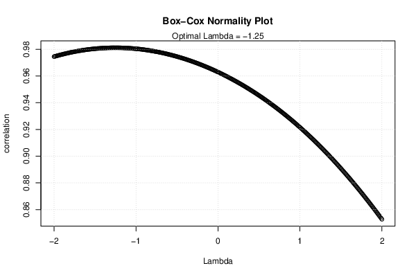
plot(l,c,main='Box-Cox Normality Plot', xlab='Lambda',ylab='correlation')
mtext(paste('Optimal Lambda =',mxli))
grid()
dev.off()
bitmap(file='test2.png')
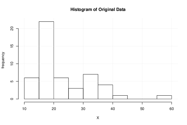
hist(x,main='Histogram of Original Data',xlab='X',ylab='frequency')
grid()
dev.off()
bitmap(file='test3.png')
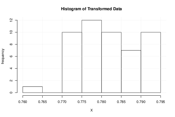
hist(x1,main='Histogram of Transformed Data', xlab='X',ylab='frequency')
grid()
dev.off()
bitmap(file='test4.png')
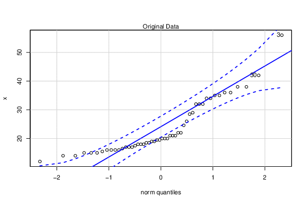
qqPlot(x)
grid()
mtext('Original Data')
dev.off()
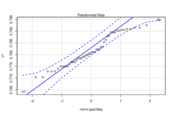
bitmap(file='test5.png')
qqPlot(x1)
grid()
mtext('Transformed Data')
dev.off()
load(file='createtable')
a<-table.start()
a<-table.row.start(a)
a<-table.element(a,'Box-Cox Normality Plot',2,TRUE)
a<-table.row.end(a)
a<-table.row.start(a)
a<-table.element(a,'# observations x',header=TRUE)
a<-table.element(a,n)
a<-table.row.end(a)
a<-table.row.start(a)
a<-table.element(a,'maximum correlation',header=TRUE)
a<-table.element(a,mx)
a<-table.row.end(a)
a<-table.row.start(a)
a<-table.element(a,'optimal lambda',header=TRUE)
a<-table.element(a,mxli)
a<-table.row.end(a)
a<-table.row.start(a)
a<-table.element(a,'transformation formula',header=TRUE)
if (par1 == 'Full Box-Cox transform') {
a<-table.element(a,'for all lambda <> 0 : T(Y) = (Y^lambda - 1) / lambda')
} else {
a<-table.element(a,'for all lambda <> 0 : T(Y) = Y^lambda')
}
a<-table.row.end(a)
if(mx<0) {
a<-table.row.start(a)
a<-table.element(a,'Warning: maximum correlation is negative! The Box-Cox transformation must not be used.',2)
a<-table.row.end(a)
}
a<-table.end(a)
table.save(a,file='mytable.tab')
if(par5=='Yes') {
a<-table.start()
a<-table.row.start(a)
a<-table.element(a,'Obs.',header=T)
a<-table.element(a,'Original',header=T)
a<-table.element(a,'Transformed',header=T)
a<-table.row.end(a)
for (i in 1:n) {
a<-table.row.start(a)
a<-table.element(a,i)
a<-table.element(a,x[i])
a<-table.element(a,x1.best[i])
a<-table.row.end(a)
}
a<-table.end(a)
table.save(a,file='mytable1.tab')
}
a<-table.start()
a<-table.row.start(a)
a<-table.element(a,'Maximum Likelihood Estimation of Lambda',1,TRUE)
a<-table.row.end(a)
a<-table.row.start(a)
a<-table.element(a,paste('
',RC.texteval('summary(mypT)'),'
',sep=''))
a<-table.row.end(a)
a<-table.end(a)
table.save(a,file='mytable3.tab')