| Multiple Linear Regression - Estimated Regression Equation |
| a[t] = -115.487 -69.3828b[t] + 230.365c[t] + 20.2521d[t] + e[t] |
| Multiple Linear Regression - Ordinary Least Squares | |||||
| Variable | Parameter | S.D. | T-STAT H0: parameter = 0 | 2-tail p-value | 1-tail p-value |
| (Intercept) | -115.5 | 26.01 | -4.4400e+00 | 3.044e-05 | 1.522e-05 |
| b | -69.38 | 56.22 | -1.2340e+00 | 0.221 | 0.1105 |
| c | +230.4 | 50.6 | +4.5530e+00 | 2.007e-05 | 1.003e-05 |
| d | +20.25 | 45.9 | +4.4120e-01 | 0.6603 | 0.3302 |
| Multiple Linear Regression - Regression Statistics | |
| Multiple R | 0.6082 |
| R-squared | 0.3699 |
| Adjusted R-squared | 0.3447 |
| F-TEST (value) | 14.68 |
| F-TEST (DF numerator) | 3 |
| F-TEST (DF denominator) | 75 |
| p-value | 1.304e-07 |
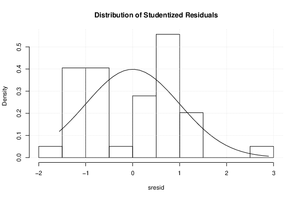
| Multiple Linear Regression - Residual Statistics | |
| Residual Standard Deviation | 11.74 |
| Sum Squared Residuals | 1.033e+04 |
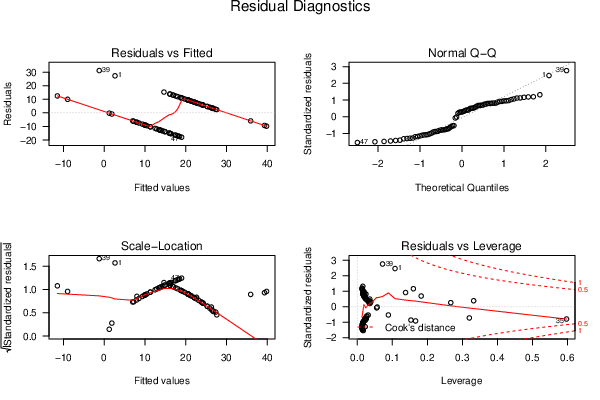
| Menu of Residual Diagnostics | |
| Description | Link |
| Histogram | Compute |
| Central Tendency | Compute |
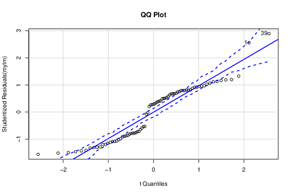
| QQ Plot | Compute |
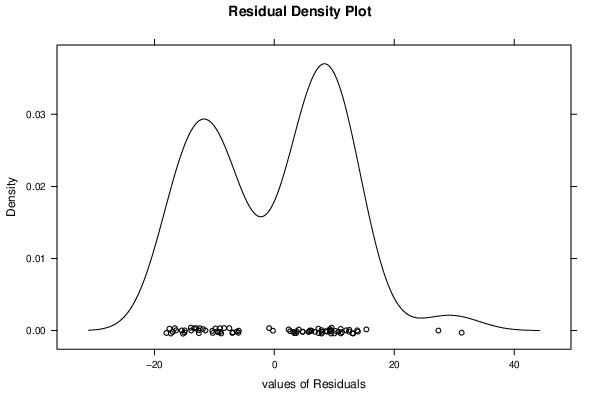
| Kernel Density Plot | Compute |
| Skewness/Kurtosis Test | Compute |
| Skewness-Kurtosis Plot | Compute |
| Harrell-Davis Plot | Compute |
| Bootstrap Plot -- Central Tendency | Compute |
| Blocked Bootstrap Plot -- Central Tendency | Compute |
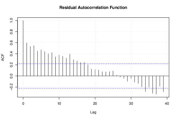
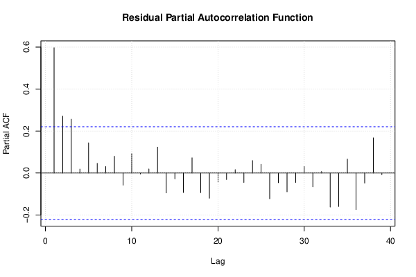
| (Partial) Autocorrelation Plot | Compute |
| Spectral Analysis | Compute |
| Tukey lambda PPCC Plot | Compute |
| Box-Cox Normality Plot | Compute |
| Summary Statistics | Compute |
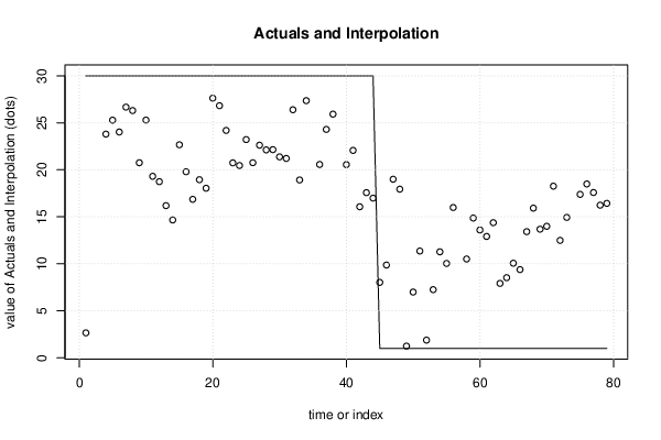
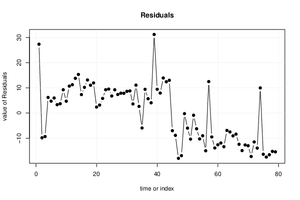
| Multiple Linear Regression - Actuals, Interpolation, and Residuals | |||
| Time or Index | Actuals | Interpolation Forecast | Residuals Prediction Error |
| 1 | 30 | 2.647 | 27.35 |
| 2 | 30 | 39.83 | -9.832 |
| 3 | 30 | 39.34 | -9.338 |
| 4 | 30 | 23.8 | 6.203 |
| 5 | 30 | 25.28 | 4.717 |
| 6 | 30 | 24.02 | 5.978 |
| 7 | 30 | 26.67 | 3.329 |
| 8 | 30 | 26.3 | 3.697 |
| 9 | 30 | 20.75 | 9.246 |
| 10 | 30 | 25.29 | 4.708 |
| 11 | 30 | 19.31 | 10.69 |
| 12 | 30 | 18.74 | 11.26 |
| 13 | 30 | 16.19 | 13.81 |
| 14 | 30 | 14.66 | 15.34 |
| 15 | 30 | 22.66 | 7.335 |
| 16 | 30 | 19.79 | 10.21 |
| 17 | 30 | 16.86 | 13.14 |
| 18 | 30 | 18.95 | 11.05 |
| 19 | 30 | 18.04 | 11.96 |
| 20 | 30 | 27.62 | 2.378 |
| 21 | 30 | 26.82 | 3.176 |
| 22 | 30 | 24.19 | 5.81 |
| 23 | 30 | 20.74 | 9.261 |
| 24 | 30 | 20.46 | 9.543 |
| 25 | 30 | 23.22 | 6.782 |
| 26 | 30 | 20.76 | 9.243 |
| 27 | 30 | 22.62 | 7.379 |
| 28 | 30 | 22.12 | 7.882 |
| 29 | 30 | 22.14 | 7.855 |
| 30 | 30 | 21.38 | 8.624 |
| 31 | 30 | 21.21 | 8.792 |
| 32 | 30 | 26.39 | 3.61 |
| 33 | 30 | 18.92 | 11.08 |
| 34 | 30 | 27.36 | 2.642 |
| 35 | 30 | 35.93 | -5.932 |
| 36 | 30 | 20.57 | 9.435 |
| 37 | 30 | 24.3 | 5.702 |
| 38 | 30 | 25.92 | 4.078 |
| 39 | 30 | -1.224 | 31.22 |
| 40 | 30 | 20.55 | 9.45 |
| 41 | 30 | 22.06 | 7.938 |
| 42 | 30 | 16.07 | 13.93 |
| 43 | 30 | 17.57 | 12.43 |
| 44 | 30 | 16.98 | 13.02 |
| 45 | 1 | 8.015 | -7.015 |
| 46 | 1 | 9.863 | -8.863 |
| 47 | 1 | 18.99 | -17.99 |
| 48 | 1 | 17.94 | -16.94 |
| 49 | 1 | 1.234 | -0.2345 |
| 50 | 1 | 6.987 | -5.987 |
| 51 | 1 | 11.36 | -10.36 |
| 52 | 1 | 1.873 | -0.8732 |
| 53 | 1 | 7.245 | -6.245 |
| 54 | 1 | 11.27 | -10.27 |
| 55 | 1 | 10.03 | -9.032 |
| 56 | 1 | 15.98 | -14.98 |
| 57 | 1 | -11.5 | 12.5 |
| 58 | 1 | 10.51 | -9.507 |
| 59 | 1 | 14.86 | -13.86 |
| 60 | 1 | 13.59 | -12.59 |
| 61 | 1 | 12.91 | -11.91 |
| 62 | 1 | 14.37 | -13.37 |
| 63 | 1 | 7.907 | -6.907 |
| 64 | 1 | 8.518 | -7.518 |
| 65 | 1 | 10.06 | -9.058 |
| 66 | 1 | 9.379 | -8.379 |
| 67 | 1 | 13.42 | -12.42 |
| 68 | 1 | 15.92 | -14.92 |
| 69 | 1 | 13.68 | -12.68 |
| 70 | 1 | 13.99 | -12.99 |
| 71 | 1 | 18.26 | -17.26 |
| 72 | 1 | 12.49 | -11.49 |
| 73 | 1 | 14.93 | -13.93 |
| 74 | 1 | -8.985 | 9.985 |
| 75 | 1 | 17.38 | -16.38 |
| 76 | 1 | 18.49 | -17.49 |
| 77 | 1 | 17.58 | -16.58 |
| 78 | 1 | 16.23 | -15.23 |
| 79 | 1 | 16.42 | -15.42 |
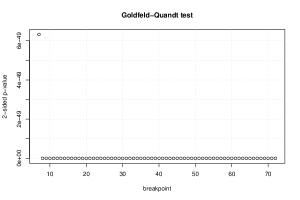
| Goldfeld-Quandt test for Heteroskedasticity | |||
| p-values | Alternative Hypothesis | ||
| breakpoint index | greater | 2-sided | less |
| 7 | 3.162e-49 | 6.323e-49 | 1 |
| 8 | 0 | 0 | 1 |
| 9 | 0 | 0 | 1 |
| 10 | 1.748e-95 | 3.496e-95 | 1 |
| 11 | 3.38e-109 | 6.76e-109 | 1 |
| 12 | 4.8e-128 | 9.599e-128 | 1 |
| 13 | 5.335e-140 | 1.067e-139 | 1 |
| 14 | 6.683e-158 | 1.337e-157 | 1 |
| 15 | 5.957e-166 | 1.191e-165 | 1 |
| 16 | 0 | 0 | 1 |
| 17 | 0 | 0 | 1 |
| 18 | 2.016e-217 | 4.032e-217 | 1 |
| 19 | 1.195e-225 | 2.39e-225 | 1 |
| 20 | 3.097e-248 | 6.195e-248 | 1 |
| 21 | 1.408e-258 | 2.817e-258 | 1 |
| 22 | 9.747e-274 | 1.949e-273 | 1 |
| 23 | 0 | 0 | 1 |
| 24 | 5.789e-296 | 1.158e-295 | 1 |
| 25 | 0 | 0 | 1 |
| 26 | 0 | 0 | 1 |
| 27 | 0 | 0 | 1 |
| 28 | 0 | 0 | 1 |
| 29 | 0 | 0 | 1 |
| 30 | 0 | 0 | 1 |
| 31 | 0 | 0 | 1 |
| 32 | 0 | 0 | 1 |
| 33 | 0 | 0 | 1 |
| 34 | 0 | 0 | 1 |
| 35 | 0 | 0 | 1 |
| 36 | 0 | 0 | 1 |
| 37 | 0 | 0 | 1 |
| 38 | 0 | 0 | 1 |
| 39 | 0 | 0 | 1 |
| 40 | 0 | 0 | 1 |
| 41 | 0 | 0 | 1 |
| 42 | 0 | 0 | 1 |
| 43 | 0 | 0 | 1 |
| 44 | 1 | 7.677e-56 | 3.839e-56 |
| 45 | 1 | 0 | 0 |
| 46 | 1 | 0 | 0 |
| 47 | 1 | 0 | 0 |
| 48 | 1 | 0 | 0 |
| 49 | 1 | 0 | 0 |
| 50 | 1 | 0 | 0 |
| 51 | 1 | 0 | 0 |
| 52 | 1 | 0 | 0 |
| 53 | 1 | 0 | 0 |
| 54 | 1 | 0 | 0 |
| 55 | 1 | 0 | 0 |
| 56 | 1 | 2.777e-306 | 1.389e-306 |
| 57 | 1 | 3.683e-288 | 1.841e-288 |
| 58 | 1 | 1.076e-272 | 5.379e-273 |
| 59 | 1 | 5.732e-256 | 2.866e-256 |
| 60 | 1 | 3.721e-247 | 1.861e-247 |
| 61 | 1 | 3.542e-227 | 1.771e-227 |
| 62 | 1 | 8.617e-215 | 4.308e-215 |
| 63 | 1 | 0 | 0 |
| 64 | 1 | 1.335e-182 | 6.674e-183 |
| 65 | 1 | 0 | 0 |
| 66 | 1 | 0 | 0 |
| 67 | 1 | 4.145e-130 | 2.073e-130 |
| 68 | 1 | 6.904e-116 | 3.452e-116 |
| 69 | 1 | 0 | 0 |
| 70 | 1 | 0 | 0 |
| 71 | 1 | 1.834e-66 | 9.17e-67 |
| 72 | 1 | 0 | 0 |
| Meta Analysis of Goldfeld-Quandt test for Heteroskedasticity | |||
| Description | # significant tests | % significant tests | OK/NOK |
| 1% type I error level | 66 | 1 | NOK |
| 5% type I error level | 66 | 1 | NOK |
| 10% type I error level | 66 | 1 | NOK |
| Ramsey RESET F-Test for powers (2 and 3) of fitted values |
> reset_test_fitted RESET test data: mylm RESET = 7.8206, df1 = 2, df2 = 73, p-value = 0.0008368 |
| Ramsey RESET F-Test for powers (2 and 3) of regressors |
> reset_test_regressors RESET test data: mylm RESET = 4.1706, df1 = 6, df2 = 69, p-value = 0.001237 |
| Ramsey RESET F-Test for powers (2 and 3) of principal components |
> reset_test_principal_components RESET test data: mylm RESET = 0.10171, df1 = 2, df2 = 73, p-value = 0.9034 |
| Variance Inflation Factors (Multicollinearity) |
> vif
       b        c        d
3.352905 3.002299 2.736238
|