Free Statistics
of Irreproducible Research!
Description of Statistical Computation | ||||||||||||||||||||||||||||||||||||||||||||||||
|---|---|---|---|---|---|---|---|---|---|---|---|---|---|---|---|---|---|---|---|---|---|---|---|---|---|---|---|---|---|---|---|---|---|---|---|---|---|---|---|---|---|---|---|---|---|---|---|---|
| Author's title | ||||||||||||||||||||||||||||||||||||||||||||||||
| Author | *Unverified author* | |||||||||||||||||||||||||||||||||||||||||||||||
| R Software Module | rwasp_fitdistrnorm.wasp | |||||||||||||||||||||||||||||||||||||||||||||||
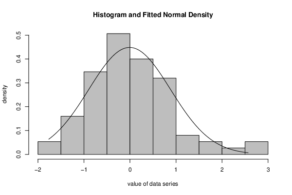
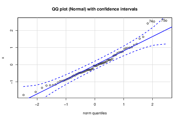
| Title produced by software | ML Fitting and QQ Plot- Normal Distribution | |||||||||||||||||||||||||||||||||||||||||||||||
| Date of computation | Sun, 14 Jun 2020 16:32:35 +0200 | |||||||||||||||||||||||||||||||||||||||||||||||
| Cite this page as follows | Statistical Computations at FreeStatistics.org, Office for Research Development and Education, URL https://freestatistics.org/blog/index.php?v=date/2020/Jun/14/t15921457017jxqlawrir149mq.htm/, Retrieved Sat, 20 Apr 2024 03:48:27 +0000 | |||||||||||||||||||||||||||||||||||||||||||||||
| Statistical Computations at FreeStatistics.org, Office for Research Development and Education, URL https://freestatistics.org/blog/index.php?pk=319176, Retrieved Sat, 20 Apr 2024 03:48:27 +0000 | ||||||||||||||||||||||||||||||||||||||||||||||||
| QR Codes: | ||||||||||||||||||||||||||||||||||||||||||||||||
|
| ||||||||||||||||||||||||||||||||||||||||||||||||
| Original text written by user: | Difference between actual and predicted loudspeaker preference scores in the Sean Olive study (generalized model): http://www.aes.org/e-lib/browse.cfm?elib=12847 (Figure 5) Figure digitized by Sancus: https://www.audiosciencereview.com/forum/index.php?threads/master-preference-ratings-for-loudspeakers.11091/page-13#post-343941 | |||||||||||||||||||||||||||||||||||||||||||||||
| IsPrivate? | No (this computation is public) | |||||||||||||||||||||||||||||||||||||||||||||||
| User-defined keywords | olive,speaker,loudspeaker,preference,rating,error | |||||||||||||||||||||||||||||||||||||||||||||||
| Estimated Impact | 214 | |||||||||||||||||||||||||||||||||||||||||||||||
Tree of Dependent Computations | ||||||||||||||||||||||||||||||||||||||||||||||||
| Family? (F = Feedback message, R = changed R code, M = changed R Module, P = changed Parameters, D = changed Data) | ||||||||||||||||||||||||||||||||||||||||||||||||
| - [ML Fitting and QQ Plot- Normal Distribution] [Olive Loudspeaker...] [2020-06-14 14:32:35] [d41d8cd98f00b204e9800998ecf8427e] [Current] | ||||||||||||||||||||||||||||||||||||||||||||||||
| Feedback Forum | ||||||||||||||||||||||||||||||||||||||||||||||||
Post a new message | ||||||||||||||||||||||||||||||||||||||||||||||||
Dataset | ||||||||||||||||||||||||||||||||||||||||||||||||
| Dataseries X: | ||||||||||||||||||||||||||||||||||||||||||||||||
-1.766 -1.587 -1.349 -1.216 -1.202 -1.191 -1.148 -1.037 -0.972 -0.954 -0.9249 -0.889 -0.845 -0.81 -0.764 -0.738 -0.67 -0.628 -0.626 -0.561 -0.546 -0.485 -0.479 -0.46 -0.449 -0.417 -0.399 -0.376 -0.334 -0.325 -0.296 -0.296 -0.293 -0.29 -0.242 -0.214 -0.065 -0.062 -0.06 -0.059 0.005 0.018 0.05 0.051 0.083 0.091 0.118 0.134 0.158 0.193 0.266 0.274 0.285 0.29 0.349 0.506 0.561 0.564 0.649 0.695 0.726 0.741 0.771 0.915 0.969 0.976 0.992 1.022 1.149 1.211 1.52 1.623 2.406 2.518 2.568 | ||||||||||||||||||||||||||||||||||||||||||||||||
Tables (Output of Computation) | ||||||||||||||||||||||||||||||||||||||||||||||||
| ||||||||||||||||||||||||||||||||||||||||||||||||
Figures (Output of Computation) | ||||||||||||||||||||||||||||||||||||||||||||||||
Input Parameters & R Code | ||||||||||||||||||||||||||||||||||||||||||||||||
| Parameters (Session): | ||||||||||||||||||||||||||||||||||||||||||||||||
| Parameters (R input): | ||||||||||||||||||||||||||||||||||||||||||||||||
| par1 = 8 ; par2 = 0 ; | ||||||||||||||||||||||||||||||||||||||||||||||||
| R code (references can be found in the software module): | ||||||||||||||||||||||||||||||||||||||||||||||||
par2 <- '0' | ||||||||||||||||||||||||||||||||||||||||||||||||