| Multiple Linear Regression - Estimated Regression Equation |
| verkoop[t] = + 190.67 + 0.419366winkels[t] + 2.22225advertenties[t] + 0.592604influencers[t] + e[t] |
| Multiple Linear Regression - Ordinary Least Squares | |||||
| Variable | Parameter | S.D. | T-STAT H0: parameter = 0 | 2-tail p-value | 1-tail p-value |
| (Intercept) | +190.7 | 42.49 | +4.4870e+00 | 0.0001531 | 7.657e-05 |
| winkels | +0.4194 | 0.157 | +2.6710e+00 | 0.01336 | 0.00668 |
| advertenties | +2.222 | 1.596 | +1.3920e+00 | 0.1766 | 0.0883 |
| influencers | +0.5926 | 0.1203 | +4.9250e+00 | 5.032e-05 | 2.516e-05 |
| Multiple Linear Regression - Regression Statistics | |
| Multiple R | 0.8186 |
| R-squared | 0.6701 |
| Adjusted R-squared | 0.6289 |
| F-TEST (value) | 16.25 |
| F-TEST (DF numerator) | 3 |
| F-TEST (DF denominator) | 24 |
| p-value | 5.575e-06 |
| Multiple Linear Regression - Residual Statistics | |
| Residual Standard Deviation | 60.25 |
| Sum Squared Residuals | 8.712e+04 |
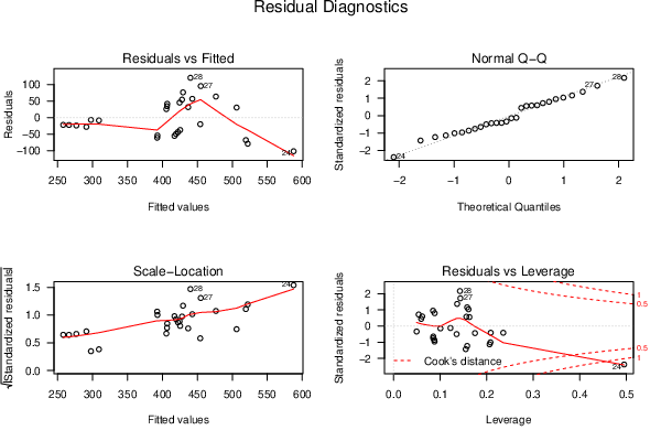
| Menu of Residual Diagnostics | |
| Description | Link |
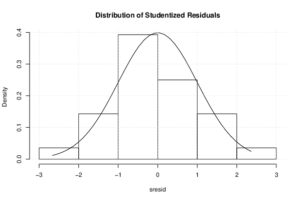
| Histogram | Compute |
| Central Tendency | Compute |
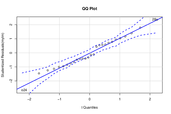
| QQ Plot | Compute |
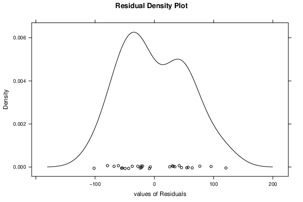
| Kernel Density Plot | Compute |
| Skewness/Kurtosis Test | Compute |
| Skewness-Kurtosis Plot | Compute |
| Harrell-Davis Plot | Compute |
| Bootstrap Plot -- Central Tendency | Compute |
| Blocked Bootstrap Plot -- Central Tendency | Compute |
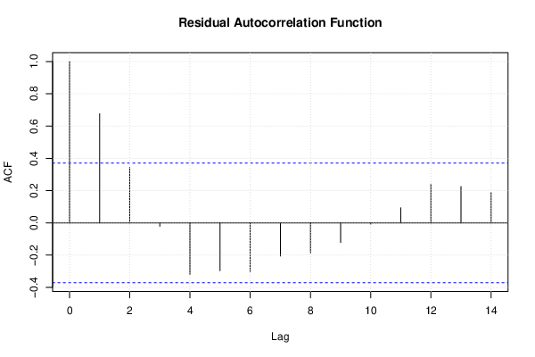
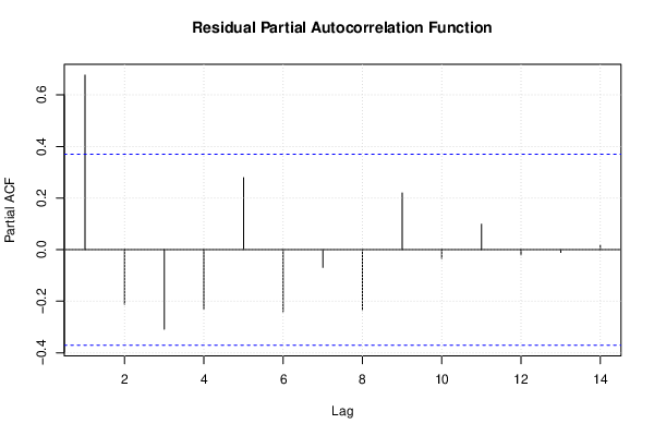
| (Partial) Autocorrelation Plot | Compute |
| Spectral Analysis | Compute |
| Tukey lambda PPCC Plot | Compute |
| Box-Cox Normality Plot | Compute |
| Summary Statistics | Compute |
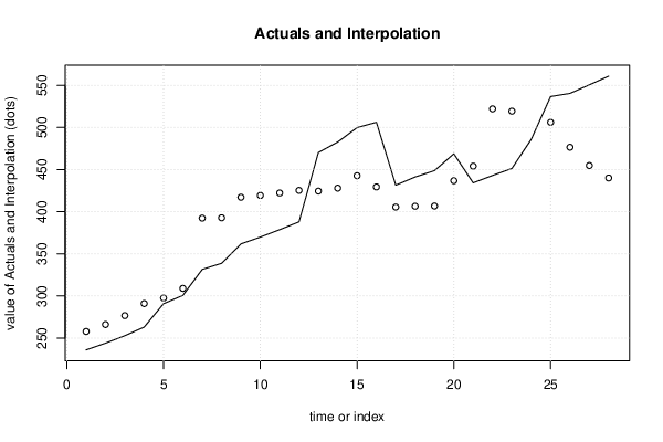
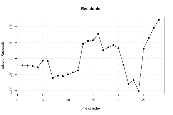
| Multiple Linear Regression - Actuals, Interpolation, and Residuals | |||
| Time or Index | Actuals | Interpolation Forecast | Residuals Prediction Error |
| 1 | 236 | 257.9 | -21.86 |
| 2 | 244 | 266.1 | -22.15 |
| 3 | 252.9 | 276.7 | -23.85 |
| 4 | 263.1 | 291 | -27.94 |
| 5 | 290.8 | 297.6 | -6.789 |
| 6 | 300.7 | 309 | -8.294 |
| 7 | 331.6 | 392.4 | -60.78 |
| 8 | 338.8 | 392.8 | -53.99 |
| 9 | 361.8 | 417.2 | -55.34 |
| 10 | 369.9 | 419.3 | -49.45 |
| 11 | 378.7 | 422.2 | -43.5 |
| 12 | 387.9 | 425.3 | -37.33 |
| 13 | 470.2 | 424.5 | 45.73 |
| 14 | 482.7 | 428 | 54.71 |
| 15 | 499.8 | 442.7 | 57.1 |
| 16 | 506.1 | 429.4 | 76.7 |
| 17 | 431.5 | 405.5 | 25.95 |
| 18 | 441.2 | 406.5 | 34.67 |
| 19 | 448.7 | 406.8 | 41.96 |
| 20 | 468.7 | 436.8 | 31.95 |
| 21 | 434.3 | 454.1 | -19.81 |
| 22 | 443 | 522 | -79.02 |
| 23 | 451.3 | 519.3 | -68 |
| 24 | 486 | 587.7 | -101.8 |
| 25 | 536.7 | 506.1 | 30.61 |
| 26 | 540.4 | 476.5 | 63.95 |
| 27 | 550.5 | 454.8 | 95.74 |
| 28 | 560.8 | 440 | 120.8 |
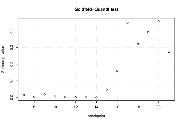
| Goldfeld-Quandt test for Heteroskedasticity | |||
| p-values | Alternative Hypothesis | ||
| breakpoint index | greater | 2-sided | less |
| 7 | 0.00704 | 0.01408 | 0.993 |
| 8 | 0.001444 | 0.002889 | 0.9986 |
| 9 | 0.009 | 0.018 | 0.991 |
| 10 | 0.002903 | 0.005806 | 0.9971 |
| 11 | 0.001031 | 0.002061 | 0.999 |
| 12 | 0.0004688 | 0.0009376 | 0.9995 |
| 13 | 0.0001331 | 0.0002661 | 0.9999 |
| 14 | 5.231e-05 | 0.0001046 | 0.9999 |
| 15 | 0.02356 | 0.04713 | 0.9764 |
| 16 | 0.08033 | 0.1607 | 0.9197 |
| 17 | 0.2246 | 0.4492 | 0.7754 |
| 18 | 0.1604 | 0.3207 | 0.8396 |
| 19 | 0.1964 | 0.3927 | 0.8036 |
| 20 | 0.2295 | 0.459 | 0.7705 |
| 21 | 0.1375 | 0.275 | 0.8625 |
| Meta Analysis of Goldfeld-Quandt test for Heteroskedasticity | |||
| Description | # significant tests | % significant tests | OK/NOK |
| 1% type I error level | 6 | 0.4 | NOK |
| 5% type I error level | 9 | 0.6 | NOK |
| 10% type I error level | 9 | 0.6 | NOK |
| Ramsey RESET F-Test for powers (2 and 3) of fitted values |
> reset_test_fitted RESET test data: mylm RESET = 24.193, df1 = 2, df2 = 22, p-value = 2.781e-06 |
| Ramsey RESET F-Test for powers (2 and 3) of regressors |
> reset_test_regressors RESET test data: mylm RESET = 16.631, df1 = 6, df2 = 18, p-value = 1.861e-06 |
| Ramsey RESET F-Test for powers (2 and 3) of principal components |
> reset_test_principal_components RESET test data: mylm RESET = 12.252, df1 = 2, df2 = 22, p-value = 0.0002656 |
| Variance Inflation Factors (Multicollinearity) |
> vif
     winkels advertenties  influencers
    1.713016     1.907646     1.234221
|