| Multiple Linear Regression - Estimated Regression Equation |
| SP[t] = -250.155 + 73.3043V[t] -0.171478SQ[t] + 27.6031BR[t] -78.6611PH[t] + 50.6011GR[t] -6.22991PK[t] + 8.44973AG[t] + 82.5753Re[t] + 1.15958As[t] + 137.4C[t] -25.7549TH[t] + e[t] |
| Multiple Linear Regression - Ordinary Least Squares | |||||
| Variable | Parameter | S.D. | T-STAT H0: parameter = 0 | 2-tail p-value | 1-tail p-value |
| (Intercept) | -250.2 | 103.1 | -2.4270e+00 | 0.02597 | 0.01298 |
| V | +73.3 | 49.59 | +1.4780e+00 | 0.1567 | 0.07834 |
| SQ | -0.1715 | 0.09469 | -1.8110e+00 | 0.08687 | 0.04343 |
| BR | +27.6 | 45.97 | +6.0050e-01 | 0.5556 | 0.2778 |
| PH | -78.66 | 47.75 | -1.6470e+00 | 0.1168 | 0.05842 |
| GR | +50.6 | 50.83 | +9.9540e-01 | 0.3327 | 0.1664 |
| PK | -6.23 | 46.29 | -1.3460e-01 | 0.8944 | 0.4472 |
| AG | +8.45 | 3.18 | +2.6570e+00 | 0.01605 | 0.008023 |
| Re | +82.58 | 48.56 | +1.7010e+00 | 0.1062 | 0.05312 |
| As | +1.16 | 0.1378 | +8.4140e+00 | 1.185e-07 | 5.925e-08 |
| C | +137.4 | 42.22 | +3.2540e+00 | 0.004405 | 0.002202 |
| TH | -25.75 | 70.41 | -3.6580e-01 | 0.7188 | 0.3594 |
| Multiple Linear Regression - Regression Statistics | |
| Multiple R | 0.9833 |
| R-squared | 0.9669 |
| Adjusted R-squared | 0.9467 |
| F-TEST (value) | 47.86 |
| F-TEST (DF numerator) | 11 |
| F-TEST (DF denominator) | 18 |
| p-value | 5.011e-11 |
| Multiple Linear Regression - Residual Statistics | |
| Residual Standard Deviation | 77.03 |
| Sum Squared Residuals | 1.068e+05 |
| Menu of Residual Diagnostics | |
| Description | Link |
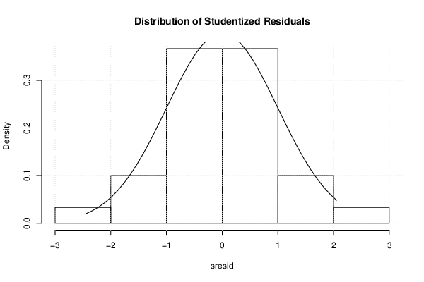
| Histogram | Compute |
| Central Tendency | Compute |
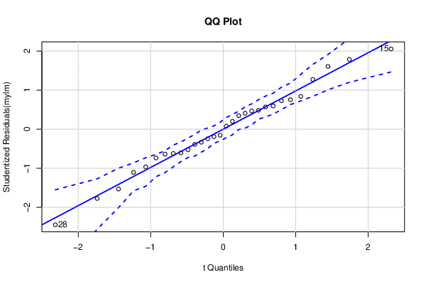
| QQ Plot | Compute |
| Kernel Density Plot | Compute |
| Skewness/Kurtosis Test | Compute |
| Skewness-Kurtosis Plot | Compute |
| Harrell-Davis Plot | Compute |
| Bootstrap Plot -- Central Tendency | Compute |
| Blocked Bootstrap Plot -- Central Tendency | Compute |
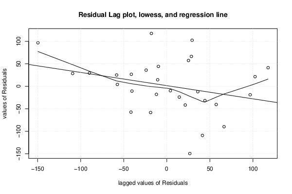
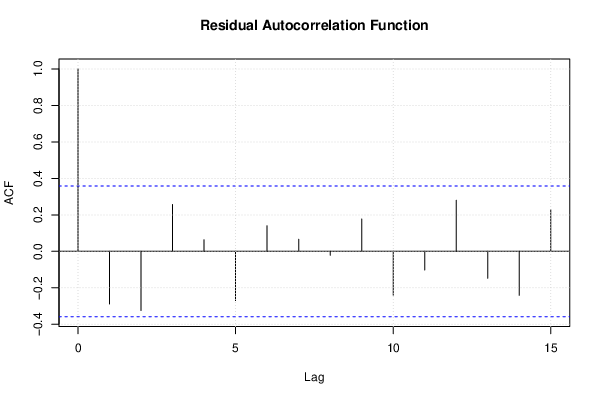
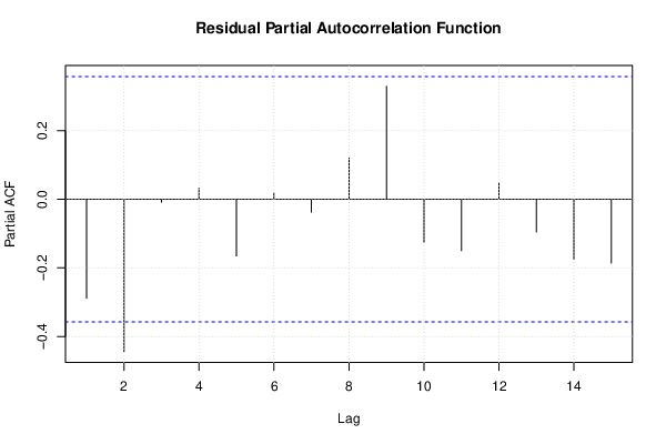
| (Partial) Autocorrelation Plot | Compute |
| Spectral Analysis | Compute |
| Tukey lambda PPCC Plot | Compute |
| Box-Cox Normality Plot | Compute |
| Summary Statistics | Compute |
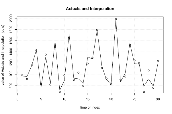
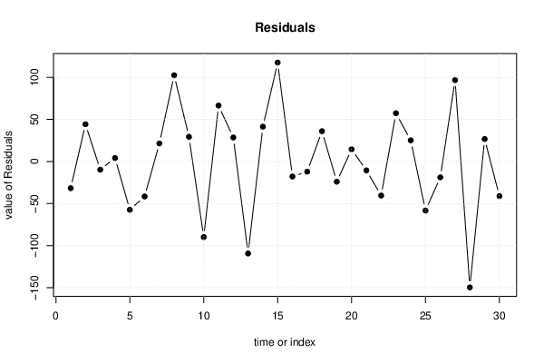
| Multiple Linear Regression - Actuals, Interpolation, and Residuals | |||
| Time or Index | Actuals | Interpolation Forecast | Residuals Prediction Error |
| 1 | 955 | 986.7 | -31.73 |
| 2 | 960 | 915.7 | 44.27 |
| 3 | 1156 | 1166 | -9.75 |
| 4 | 1433 | 1429 | 4.177 |
| 5 | 769 | 826.4 | -57.38 |
| 6 | 1310 | 1352 | -41.58 |
| 7 | 840 | 818.5 | 21.45 |
| 8 | 1590 | 1488 | 102.4 |
| 9 | 716 | 686.6 | 29.36 |
| 10 | 892 | 981.8 | -89.84 |
| 11 | 1717 | 1651 | 66.46 |
| 12 | 930 | 901.5 | 28.52 |
| 13 | 920 | 1029 | -109.3 |
| 14 | 838 | 796.6 | 41.39 |
| 15 | 1310 | 1192 | 117.6 |
| 16 | 1275 | 1293 | -17.88 |
| 17 | 1780 | 1792 | -12.03 |
| 18 | 1148 | 1112 | 36.01 |
| 19 | 900 | 924 | -23.98 |
| 20 | 839 | 824.5 | 14.5 |
| 21 | 1975 | 1986 | -10.56 |
| 22 | 865 | 905.4 | -40.42 |
| 23 | 1018 | 960.7 | 57.35 |
| 24 | 1550 | 1525 | 25.15 |
| 25 | 1190 | 1248 | -58.24 |
| 26 | 1182 | 1201 | -18.76 |
| 27 | 783 | 686.2 | 96.77 |
| 28 | 920 | 1070 | -149.6 |
| 29 | 788 | 761.2 | 26.76 |
| 30 | 1193 | 1234 | -41.16 |
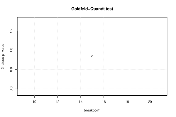
| Goldfeld-Quandt test for Heteroskedasticity | |||
| p-values | Alternative Hypothesis | ||
| breakpoint index | greater | 2-sided | less |
| 15 | 0.4679 | 0.9359 | 0.5321 |
| Meta Analysis of Goldfeld-Quandt test for Heteroskedasticity | |||
| Description | # significant tests | % significant tests | OK/NOK |
| 1% type I error level | 0 | 0 | OK |
| 5% type I error level | 0 | 0 | OK |
| 10% type I error level | 0 | 0 | OK |
| Ramsey RESET F-Test for powers (2 and 3) of fitted values |
> reset_test_fitted RESET test data: mylm RESET = 7.285, df1 = 2, df2 = 16, p-value = 0.005631 |
| Ramsey RESET F-Test for powers (2 and 3) of regressors |
> reset_test_regressors RESET test data: mylm RESET = -0.36952, df1 = 22, df2 = -4, p-value = NA |
| Ramsey RESET F-Test for powers (2 and 3) of principal components |
> reset_test_principal_components RESET test data: mylm RESET = 0.3125, df1 = 2, df2 = 16, p-value = 0.736 |
| Variance Inflation Factors (Multicollinearity) |
> vif
        V        SQ        BR        PH        GR        PK        AG        Re
 1.639363 17.057586  3.335171  1.601112  1.509764  2.696835  3.891731  2.400751
       As         C        TH
10.963412  2.243383  2.896230
|