| Multiple Linear Regression - Estimated Regression Equation |
| SP[t] = -206.511 + 71.2444V[t] -0.183629SQ[t] + 26.824BR[t] -93.3207PH[t] + 26.2094GR[t] + 6.69124AG[t] + 103.934Re[t] + 1.17563As[t] + 114.936C[t] + 0.070718D[t] -0.891816T[t] + e[t] |
| Multiple Linear Regression - Ordinary Least Squares | |||||
| Variable | Parameter | S.D. | T-STAT H0: parameter = 0 | 2-tail p-value | 1-tail p-value |
| (Intercept) | -206.5 | 121 | -1.7060e+00 | 0.1051 | 0.05257 |
| V | +71.24 | 48.36 | +1.4730e+00 | 0.158 | 0.079 |
| SQ | -0.1836 | 0.09138 | -2.0090e+00 | 0.05973 | 0.02987 |
| BR | +26.82 | 38.03 | +7.0530e-01 | 0.4897 | 0.2448 |
| PH | -93.32 | 46.8 | -1.9940e+00 | 0.06151 | 0.03075 |
| GR | +26.21 | 55.6 | +4.7140e-01 | 0.643 | 0.3215 |
| AG | +6.691 | 4.1 | +1.6320e+00 | 0.1201 | 0.06003 |
| Re | +103.9 | 50.07 | +2.0760e+00 | 0.05253 | 0.02627 |
| As | +1.176 | 0.1371 | +8.5740e+00 | 9.003e-08 | 4.501e-08 |
| C | +114.9 | 47.29 | +2.4300e+00 | 0.02576 | 0.01288 |
| D | +0.07072 | 0.2369 | +2.9850e-01 | 0.7688 | 0.3844 |
| T | -0.8918 | 1.199 | -7.4400e-01 | 0.4665 | 0.2332 |
| Multiple Linear Regression - Regression Statistics | |
| Multiple R | 0.9837 |
| R-squared | 0.9677 |
| Adjusted R-squared | 0.948 |
| F-TEST (value) | 49.06 |
| F-TEST (DF numerator) | 11 |
| F-TEST (DF denominator) | 18 |
| p-value | 4.049e-11 |
| Multiple Linear Regression - Residual Statistics | |
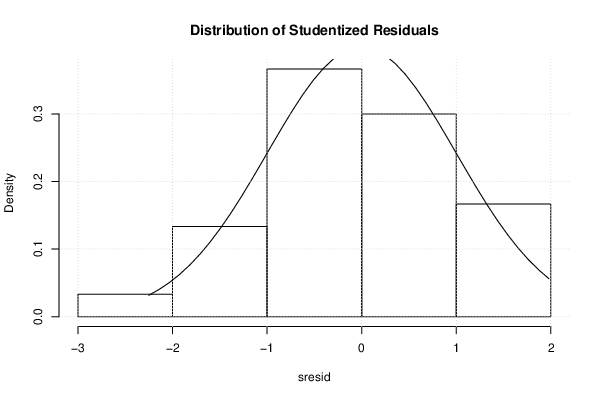
| Residual Standard Deviation | 76.11 |
| Sum Squared Residuals | 1.043e+05 |
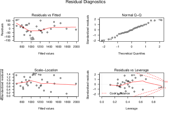
| Menu of Residual Diagnostics | |
| Description | Link |
| Histogram | Compute |
| Central Tendency | Compute |
| QQ Plot | Compute |
| Kernel Density Plot | Compute |
| Skewness/Kurtosis Test | Compute |
| Skewness-Kurtosis Plot | Compute |
| Harrell-Davis Plot | Compute |
| Bootstrap Plot -- Central Tendency | Compute |
| Blocked Bootstrap Plot -- Central Tendency | Compute |
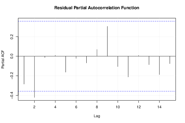
| (Partial) Autocorrelation Plot | Compute |
| Spectral Analysis | Compute |
| Tukey lambda PPCC Plot | Compute |
| Box-Cox Normality Plot | Compute |
| Summary Statistics | Compute |
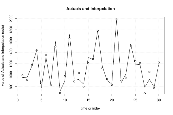
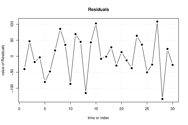
| Multiple Linear Regression - Actuals, Interpolation, and Residuals | |||
| Time or Index | Actuals | Interpolation Forecast | Residuals Prediction Error |
| 1 | 955 | 995.2 | -40.22 |
| 2 | 960 | 913.2 | 46.81 |
| 3 | 1156 | 1174 | -18 |
| 4 | 1433 | 1437 | -3.622 |
| 5 | 769 | 849.4 | -80.41 |
| 6 | 1310 | 1358 | -47.75 |
| 7 | 840 | 822 | 17.96 |
| 8 | 1590 | 1505 | 85.31 |
| 9 | 716 | 680.6 | 35.42 |
| 10 | 892 | 978.5 | -86.45 |
| 11 | 1717 | 1648 | 68.98 |
| 12 | 930 | 885.1 | 44.92 |
| 13 | 920 | 1035 | -114.8 |
| 14 | 838 | 794.7 | 43.26 |
| 15 | 1310 | 1208 | 102.2 |
| 16 | 1275 | 1283 | -7.981 |
| 17 | 1780 | 1781 | -1.172 |
| 18 | 1148 | 1120 | 27.83 |
| 19 | 900 | 929 | -29.05 |
| 20 | 839 | 826.2 | 12.8 |
| 21 | 1975 | 1988 | -13.05 |
| 22 | 865 | 902.2 | -37.21 |
| 23 | 1018 | 954.1 | 63.86 |
| 24 | 1550 | 1514 | 36.14 |
| 25 | 1190 | 1240 | -50.25 |
| 26 | 1182 | 1208 | -26.11 |
| 27 | 783 | 674.7 | 108.3 |
| 28 | 920 | 1053 | -133.4 |
| 29 | 788 | 765.2 | 22.76 |
| 30 | 1193 | 1220 | -27.01 |
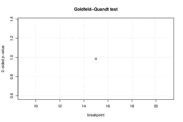
| Goldfeld-Quandt test for Heteroskedasticity | |||
| p-values | Alternative Hypothesis | ||
| breakpoint index | greater | 2-sided | less |
| 15 | 0.507 | 0.986 | 0.493 |
| Meta Analysis of Goldfeld-Quandt test for Heteroskedasticity | |||
| Description | # significant tests | % significant tests | OK/NOK |
| 1% type I error level | 0 | 0 | OK |
| 5% type I error level | 0 | 0 | OK |
| 10% type I error level | 0 | 0 | OK |
| Ramsey RESET F-Test for powers (2 and 3) of fitted values |
> reset_test_fitted RESET test data: mylm RESET = 9.8246, df1 = 2, df2 = 16, p-value = 0.001646 |
| Ramsey RESET F-Test for powers (2 and 3) of regressors |
> reset_test_regressors RESET test data: mylm RESET = -3.0668, df1 = 22, df2 = -4, p-value = NA |
| Ramsey RESET F-Test for powers (2 and 3) of principal components |
> reset_test_principal_components RESET test data: mylm RESET = 0.53896, df1 = 2, df2 = 16, p-value = 0.5936 |
| Variance Inflation Factors (Multicollinearity) |
> vif
        V        SQ        BR        PH        GR        AG        Re        As
 1.596850 16.275041  2.339137  1.575250  1.849797  6.627072  2.615194 11.116284
        C         D         T
 2.882554  1.529650  2.534818
|