| Multiple Linear Regression - Estimated Regression Equation |
| SP[t] = -178.397 + 69.2751V[t] -0.175723SQ[t] + 25.7879BR[t] -100.782PH[t] + 6.02176AG[t] + 105.971Re[t] + 1.17152As[t] + 105.094C[t] -1.16872T[t] + e[t] |
| Multiple Linear Regression - Ordinary Least Squares | |||||
| Variable | Parameter | S.D. | T-STAT H0: parameter = 0 | 2-tail p-value | 1-tail p-value |
| (Intercept) | -178.4 | 105.4 | -1.6930e+00 | 0.106 | 0.05299 |
| V | +69.28 | 44.05 | +1.5730e+00 | 0.1315 | 0.06574 |
| SQ | -0.1757 | 0.08091 | -2.1720e+00 | 0.04208 | 0.02104 |
| BR | +25.79 | 35.95 | +7.1720e-01 | 0.4815 | 0.2408 |
| PH | -100.8 | 41.47 | -2.4300e+00 | 0.02462 | 0.01231 |
| AG | +6.022 | 3.747 | +1.6070e+00 | 0.1237 | 0.06186 |
| Re | +106 | 45.24 | +2.3430e+00 | 0.02961 | 0.01481 |
| As | +1.171 | 0.127 | +9.2240e+00 | 1.209e-08 | 6.043e-09 |
| C | +105.1 | 39.14 | +2.6850e+00 | 0.01423 | 0.007114 |
| T | -1.169 | 0.9968 | -1.1720e+00 | 0.2548 | 0.1274 |
| Multiple Linear Regression - Regression Statistics | |
| Multiple R | 0.9834 |
| R-squared | 0.9672 |
| Adjusted R-squared | 0.9524 |
| F-TEST (value) | 65.45 |
| F-TEST (DF numerator) | 9 |
| F-TEST (DF denominator) | 20 |
| p-value | 7.178e-13 |
| Multiple Linear Regression - Residual Statistics | |
| Residual Standard Deviation | 72.83 |
| Sum Squared Residuals | 1.061e+05 |
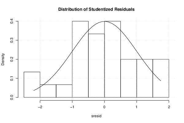
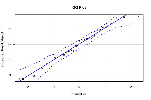
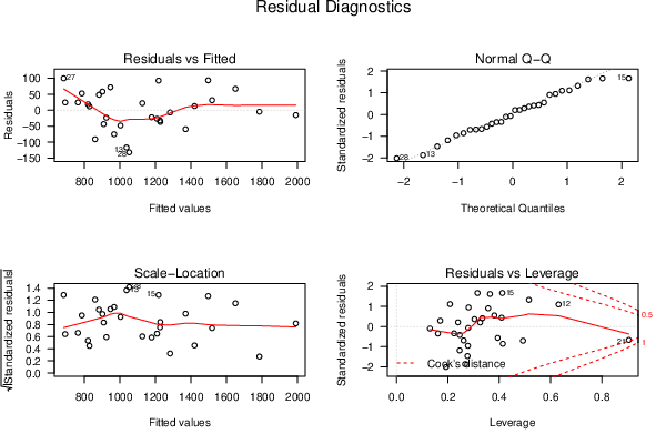
| Menu of Residual Diagnostics | |
| Description | Link |
| Histogram | Compute |
| Central Tendency | Compute |
| QQ Plot | Compute |
| Kernel Density Plot | Compute |
| Skewness/Kurtosis Test | Compute |
| Skewness-Kurtosis Plot | Compute |
| Harrell-Davis Plot | Compute |
| Bootstrap Plot -- Central Tendency | Compute |
| Blocked Bootstrap Plot -- Central Tendency | Compute |
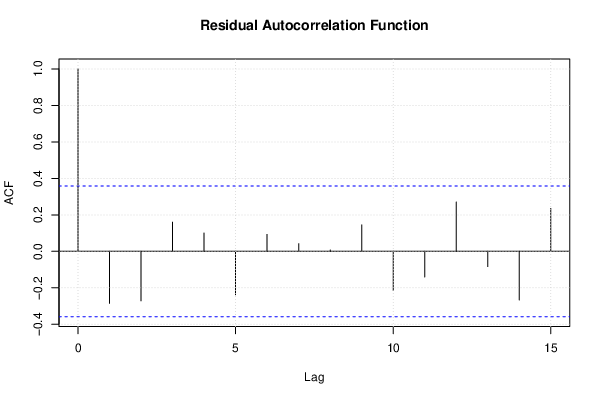
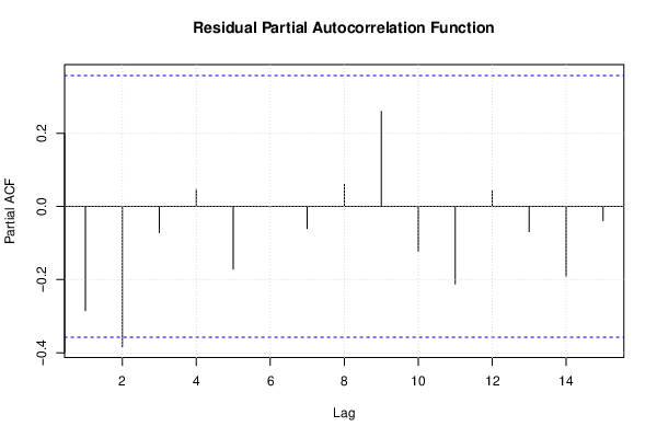
| (Partial) Autocorrelation Plot | Compute |
| Spectral Analysis | Compute |
| Tukey lambda PPCC Plot | Compute |
| Box-Cox Normality Plot | Compute |
| Summary Statistics | Compute |
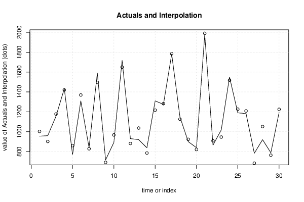
| Multiple Linear Regression - Actuals, Interpolation, and Residuals | |||
| Time or Index | Actuals | Interpolation Forecast | Residuals Prediction Error |
| 1 | 955 | 1003 | -47.86 |
| 2 | 960 | 901.5 | 58.54 |
| 3 | 1156 | 1178 | -21.98 |
| 4 | 1433 | 1420 | 13.14 |
| 5 | 769 | 859.9 | -90.91 |
| 6 | 1310 | 1369 | -59.34 |
| 7 | 840 | 828 | 11.98 |
| 8 | 1590 | 1496 | 93.79 |
| 9 | 716 | 691.6 | 24.43 |
| 10 | 892 | 967.2 | -75.16 |
| 11 | 1717 | 1650 | 67.1 |
| 12 | 930 | 881.5 | 48.45 |
| 13 | 920 | 1037 | -116.7 |
| 14 | 838 | 785.1 | 52.86 |
| 15 | 1310 | 1217 | 92.92 |
| 16 | 1275 | 1282 | -6.996 |
| 17 | 1780 | 1785 | -4.517 |
| 18 | 1148 | 1126 | 22.21 |
| 19 | 900 | 923.4 | -23.36 |
| 20 | 839 | 820.1 | 18.88 |
| 21 | 1975 | 1990 | -15.06 |
| 22 | 865 | 908.4 | -43.36 |
| 23 | 1018 | 945.9 | 72.05 |
| 24 | 1550 | 1518 | 31.5 |
| 25 | 1190 | 1227 | -36.69 |
| 26 | 1182 | 1209 | -26.63 |
| 27 | 783 | 682.8 | 100.2 |
| 28 | 920 | 1052 | -131.8 |
| 29 | 788 | 763.5 | 24.51 |
| 30 | 1193 | 1225 | -32.2 |
| Goldfeld-Quandt test for Heteroskedasticity | |||
| p-values | Alternative Hypothesis | ||
| breakpoint index | greater | 2-sided | less |
| 13 | 0.7982 | 0.4036 | 0.2018 |
| 14 | 0.6754 | 0.6491 | 0.3246 |
| 15 | 0.546 | 0.9081 | 0.454 |
| 16 | 0.4613 | 0.9225 | 0.5387 |
| 17 | 0.3492 | 0.6983 | 0.6508 |
| Meta Analysis of Goldfeld-Quandt test for Heteroskedasticity | |||
| Description | # significant tests | % significant tests | OK/NOK |
| 1% type I error level | 0 | 0 | OK |
| 5% type I error level | 0 | 0 | OK |
| 10% type I error level | 0 | 0 | OK |
| Ramsey RESET F-Test for powers (2 and 3) of fitted values |
> reset_test_fitted RESET test data: mylm RESET = 9.0364, df1 = 2, df2 = 18, p-value = 0.001918 |
| Ramsey RESET F-Test for powers (2 and 3) of regressors |
> reset_test_regressors RESET test data: mylm RESET = 1.241, df1 = 18, df2 = 2, p-value = 0.5378 |
| Ramsey RESET F-Test for powers (2 and 3) of principal components |
> reset_test_principal_components RESET test data: mylm RESET = 0.64159, df1 = 2, df2 = 18, p-value = 0.5381 |
| Variance Inflation Factors (Multicollinearity) |
> vif
        V        SQ        BR        PH        AG        Re        As         C
 1.446600 13.933951  2.282755  1.350788  6.044902  2.331050 10.417095  2.156168
        T
 1.914313
|