| Multiple Linear Regression - Estimated Regression Equation |
| SP[t] = -437.526 + 112.392V[t] + 1.50667SQ[t] -0.000205937SQ2[t] + 43.4069BR[t] -71.6116PH[t] -10.2263AG[t] + 108.215C[t] -260.046TH[t] + e[t] |
| Multiple Linear Regression - Ordinary Least Squares | |||||
| Variable | Parameter | S.D. | T-STAT H0: parameter = 0 | 2-tail p-value | 1-tail p-value |
| (Intercept) | -437.5 | 129.3 | -3.3830e+00 | 0.002678 | 0.001339 |
| V | +112.4 | 49.62 | +2.2650e+00 | 0.03371 | 0.01685 |
| SQ | +1.507 | 0.1468 | +1.0260e+01 | 7.536e-10 | 3.768e-10 |
| SQ2 | -0.0002059 | 2.814e-05 | -7.3190e+00 | 2.503e-07 | 1.252e-07 |
| BR | +43.41 | 40.72 | +1.0660e+00 | 0.298 | 0.149 |
| PH | -71.61 | 48.88 | -1.4650e+00 | 0.1571 | 0.07854 |
| AG | -10.23 | 2.95 | -3.4670e+00 | 0.002192 | 0.001096 |
| C | +108.2 | 44.03 | +2.4580e+00 | 0.02234 | 0.01117 |
| TH | -260.1 | 77.72 | -3.3460e+00 | 0.002926 | 0.001463 |
| Multiple Linear Regression - Regression Statistics | |
| Multiple R | 0.9733 |
| R-squared | 0.9472 |
| Adjusted R-squared | 0.928 |
| F-TEST (value) | 49.35 |
| F-TEST (DF numerator) | 8 |
| F-TEST (DF denominator) | 22 |
| p-value | 2.779e-12 |
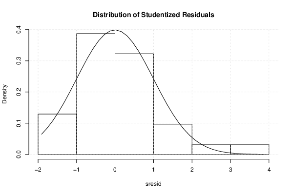
| Multiple Linear Regression - Residual Statistics | |
| Residual Standard Deviation | 88.11 |
| Sum Squared Residuals | 1.708e+05 |
| Menu of Residual Diagnostics | |
| Description | Link |
| Histogram | Compute |
| Central Tendency | Compute |
| QQ Plot | Compute |
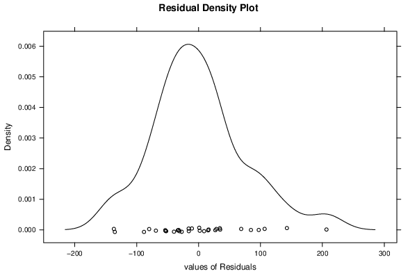
| Kernel Density Plot | Compute |
| Skewness/Kurtosis Test | Compute |
| Skewness-Kurtosis Plot | Compute |
| Harrell-Davis Plot | Compute |
| Bootstrap Plot -- Central Tendency | Compute |
| Blocked Bootstrap Plot -- Central Tendency | Compute |
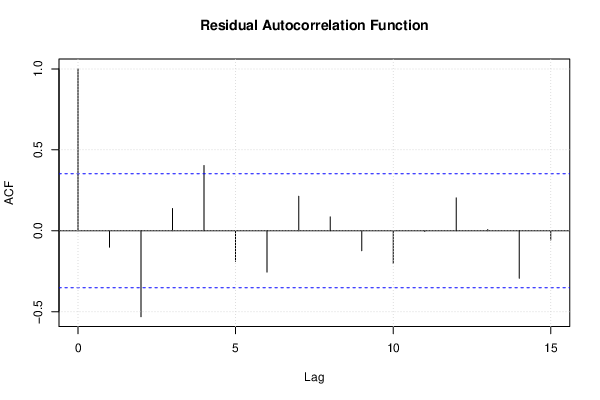
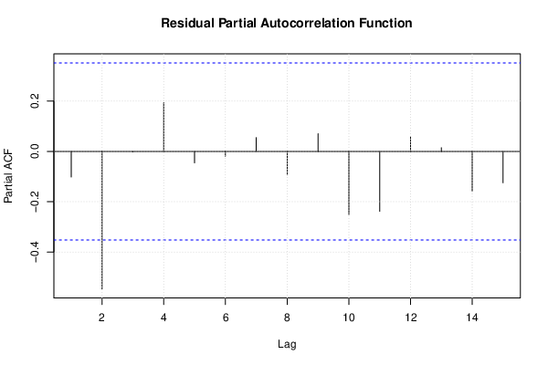
| (Partial) Autocorrelation Plot | Compute |
| Spectral Analysis | Compute |
| Tukey lambda PPCC Plot | Compute |
| Box-Cox Normality Plot | Compute |
| Summary Statistics | Compute |
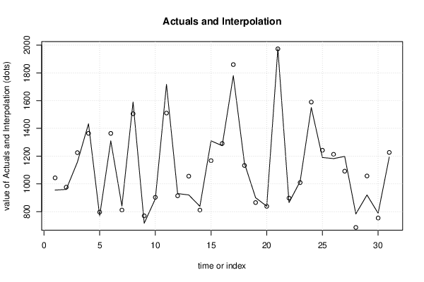
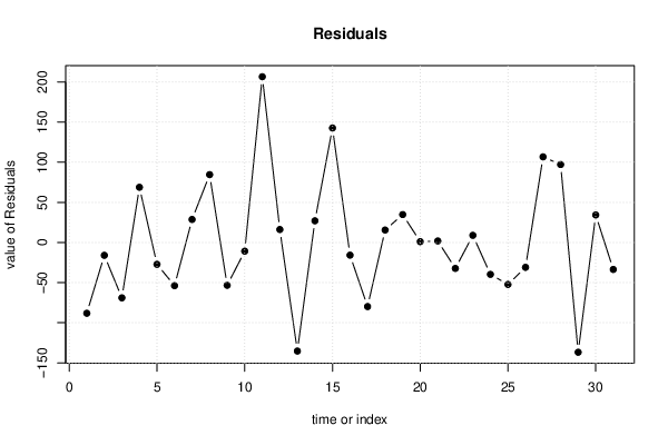
| Multiple Linear Regression - Actuals, Interpolation, and Residuals | |||
| Time or Index | Actuals | Interpolation Forecast | Residuals Prediction Error |
| 1 | 955 | 1043 | -88.18 |
| 2 | 960 | 976 | -15.99 |
| 3 | 1156 | 1225 | -68.99 |
| 4 | 1433 | 1364 | 68.81 |
| 5 | 769 | 796.2 | -27.24 |
| 6 | 1310 | 1364 | -53.8 |
| 7 | 840 | 811.3 | 28.72 |
| 8 | 1590 | 1505 | 84.57 |
| 9 | 716 | 769.4 | -53.39 |
| 10 | 892 | 902.8 | -10.79 |
| 11 | 1717 | 1510 | 206.6 |
| 12 | 930 | 913.8 | 16.17 |
| 13 | 920 | 1055 | -135.3 |
| 14 | 838 | 811 | 27.03 |
| 15 | 1310 | 1167 | 142.7 |
| 16 | 1275 | 1291 | -15.79 |
| 17 | 1780 | 1860 | -79.85 |
| 18 | 1148 | 1132 | 15.55 |
| 19 | 900 | 865.2 | 34.83 |
| 20 | 839 | 838 | 1.048 |
| 21 | 1975 | 1973 | 1.902 |
| 22 | 865 | 897.3 | -32.33 |
| 23 | 1018 | 1009 | 8.913 |
| 24 | 1550 | 1590 | -39.75 |
| 25 | 1190 | 1242 | -52.27 |
| 26 | 1182 | 1213 | -30.97 |
| 27 | 1198 | 1091 | 106.7 |
| 28 | 783 | 685.8 | 97.16 |
| 29 | 920 | 1057 | -136.8 |
| 30 | 788 | 753.7 | 34.33 |
| 31 | 1193 | 1227 | -33.57 |
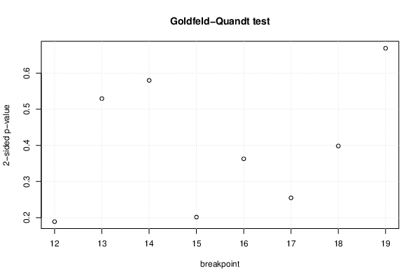
| Goldfeld-Quandt test for Heteroskedasticity | |||
| p-values | Alternative Hypothesis | ||
| breakpoint index | greater | 2-sided | less |
| 12 | 0.0944 | 0.1888 | 0.9056 |
| 13 | 0.7353 | 0.5294 | 0.2647 |
| 14 | 0.7101 | 0.5798 | 0.2899 |
| 15 | 0.8993 | 0.2014 | 0.1007 |
| 16 | 0.8186 | 0.3628 | 0.1814 |
| 17 | 0.8727 | 0.2547 | 0.1273 |
| 18 | 0.8009 | 0.3982 | 0.1991 |
| 19 | 0.6656 | 0.6688 | 0.3344 |
| Meta Analysis of Goldfeld-Quandt test for Heteroskedasticity | |||
| Description | # significant tests | % significant tests | OK/NOK |
| 1% type I error level | 0 | 0 | OK |
| 5% type I error level | 0 | 0 | OK |
| 10% type I error level | 0 | 0 | OK |
| Ramsey RESET F-Test for powers (2 and 3) of fitted values |
> reset_test_fitted RESET test data: mylm RESET = 3.1711, df1 = 2, df2 = 20, p-value = 0.06365 |
| Ramsey RESET F-Test for powers (2 and 3) of regressors |
> reset_test_regressors RESET test data: mylm RESET = 0.32075, df1 = 16, df2 = 6, p-value = 0.9678 |
| Ramsey RESET F-Test for powers (2 and 3) of principal components |
> reset_test_principal_components RESET test data: mylm RESET = 0.51573, df1 = 2, df2 = 20, p-value = 0.6048 |
| Variance Inflation Factors (Multicollinearity) |
> vif
        V        SQ       SQ2        BR        PH        AG         C        TH
 1.315653 31.548096 22.832638  2.039700  1.290921  2.729898  1.933849  2.711129
|