| Multiple Linear Regression - Estimated Regression Equation |
| DPSF[t] = + 0.943992 + 0.0549234V[t] -0.000774414SQ[t] + 7.30672e-08SQ2[t] -0.0506303PH[t] + 0.0427334GR[t] + 0.0275149Re[t] + 0.000655648As[t] + 0.096025C[t] + e[t] |
| Multiple Linear Regression - Ordinary Least Squares | |||||
| Variable | Parameter | S.D. | T-STAT H0: parameter = 0 | 2-tail p-value | 1-tail p-value |
| (Intercept) | +0.944 | 0.07466 | +1.2640e+01 | 1.448e-11 | 7.238e-12 |
| V | +0.05492 | 0.03879 | +1.4160e+00 | 0.1708 | 0.08539 |
| SQ | -0.0007744 | 0.0001465 | -5.2850e+00 | 2.65e-05 | 1.325e-05 |
| SQ2 | +7.307e-08 | 2.326e-08 | +3.1410e+00 | 0.004749 | 0.002374 |
| PH | -0.05063 | 0.03689 | -1.3730e+00 | 0.1837 | 0.09186 |
| GR | +0.04273 | 0.04153 | +1.0290e+00 | 0.3146 | 0.1573 |
| Re | +0.02752 | 0.03291 | +8.3610e-01 | 0.4121 | 0.206 |
| As | +0.0006557 | 0.000122 | +5.3720e+00 | 2.152e-05 | 1.076e-05 |
| C | +0.09602 | 0.03124 | +3.0730e+00 | 0.005561 | 0.002781 |
| Multiple Linear Regression - Regression Statistics | |
| Multiple R | 0.9451 |
| R-squared | 0.8932 |
| Adjusted R-squared | 0.8544 |
| F-TEST (value) | 23 |
| F-TEST (DF numerator) | 8 |
| F-TEST (DF denominator) | 22 |
| p-value | 5.507e-09 |
| Multiple Linear Regression - Residual Statistics | |
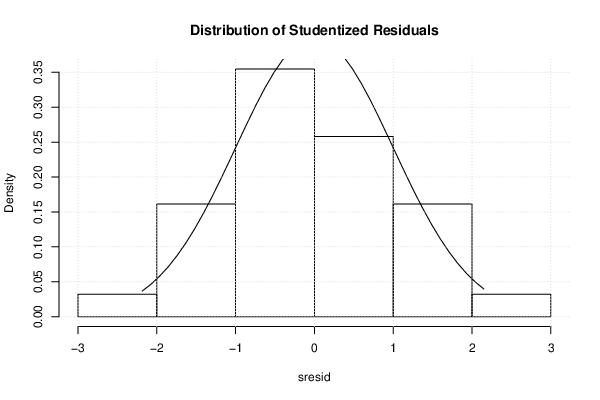
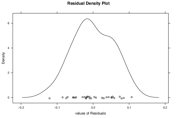
| Residual Standard Deviation | 0.06493 |
| Sum Squared Residuals | 0.09275 |
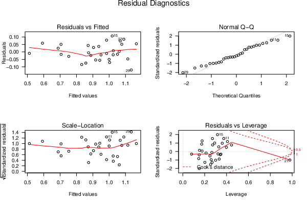
| Menu of Residual Diagnostics | |
| Description | Link |
| Histogram | Compute |
| Central Tendency | Compute |
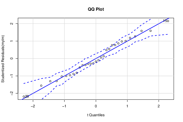
| QQ Plot | Compute |
| Kernel Density Plot | Compute |
| Skewness/Kurtosis Test | Compute |
| Skewness-Kurtosis Plot | Compute |
| Harrell-Davis Plot | Compute |
| Bootstrap Plot -- Central Tendency | Compute |
| Blocked Bootstrap Plot -- Central Tendency | Compute |
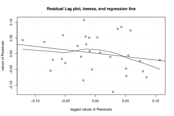
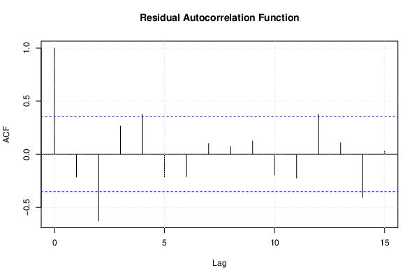
| (Partial) Autocorrelation Plot | Compute |
| Spectral Analysis | Compute |
| Tukey lambda PPCC Plot | Compute |
| Box-Cox Normality Plot | Compute |
| Summary Statistics | Compute |
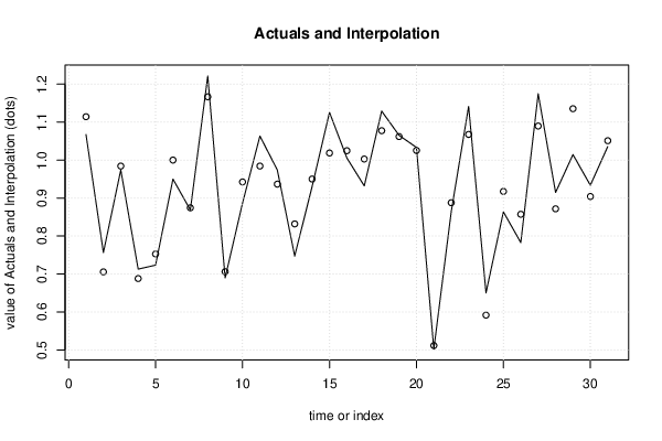
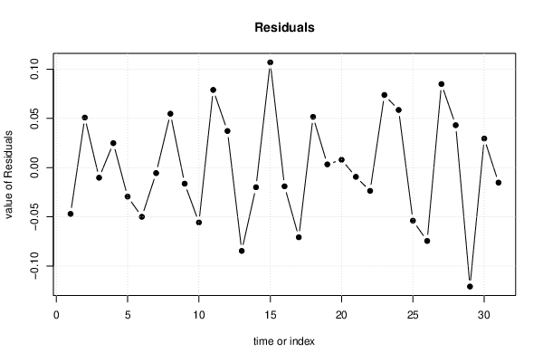
| Multiple Linear Regression - Actuals, Interpolation, and Residuals | |||
| Time or Index | Actuals | Interpolation Forecast | Residuals Prediction Error |
| 1 | 1.067 | 1.114 | -0.04703 |
| 2 | 0.7565 | 0.7057 | 0.05084 |
| 3 | 0.9739 | 0.9841 | -0.01025 |
| 4 | 0.7129 | 0.6881 | 0.02485 |
| 5 | 0.7234 | 0.7529 | -0.02943 |
| 6 | 0.95 | 0.9999 | -0.04998 |
| 7 | 0.8687 | 0.8742 | -0.005559 |
| 8 | 1.221 | 1.166 | 0.05472 |
| 9 | 0.6898 | 0.7061 | -0.01632 |
| 10 | 0.8867 | 0.9424 | -0.05575 |
| 11 | 1.063 | 0.9842 | 0.07896 |
| 12 | 0.9738 | 0.9366 | 0.03719 |
| 13 | 0.7474 | 0.832 | -0.08463 |
| 14 | 0.9301 | 0.95 | -0.01994 |
| 15 | 1.125 | 1.019 | 0.1069 |
| 16 | 1.006 | 1.025 | -0.01901 |
| 17 | 0.9319 | 1.003 | -0.07076 |
| 18 | 1.129 | 1.077 | 0.05156 |
| 19 | 1.065 | 1.062 | 0.003264 |
| 20 | 1.033 | 1.025 | 0.007972 |
| 21 | 0.5024 | 0.5118 | -0.009357 |
| 22 | 0.8641 | 0.8878 | -0.02362 |
| 23 | 1.141 | 1.067 | 0.07379 |
| 24 | 0.6504 | 0.5919 | 0.05857 |
| 25 | 0.8636 | 0.9175 | -0.0539 |
| 26 | 0.7828 | 0.8573 | -0.07451 |
| 27 | 1.175 | 1.09 | 0.08493 |
| 28 | 0.9147 | 0.8716 | 0.04311 |
| 29 | 1.014 | 1.135 | -0.1209 |
| 30 | 0.9336 | 0.9042 | 0.0295 |
| 31 | 1.036 | 1.051 | -0.01527 |
| Goldfeld-Quandt test for Heteroskedasticity | |||
| p-values | Alternative Hypothesis | ||
| breakpoint index | greater | 2-sided | less |
| 12 | 0.2882 | 0.5764 | 0.7118 |
| 13 | 0.353 | 0.7061 | 0.647 |
| 14 | 0.2378 | 0.4756 | 0.7622 |
| 15 | 0.4514 | 0.9028 | 0.5486 |
| 16 | 0.2958 | 0.5916 | 0.7042 |
| 17 | 0.2174 | 0.4348 | 0.7826 |
| 18 | 0.2981 | 0.5962 | 0.7019 |
| 19 | 0.1794 | 0.3589 | 0.8206 |
| Meta Analysis of Goldfeld-Quandt test for Heteroskedasticity | |||
| Description | # significant tests | % significant tests | OK/NOK |
| 1% type I error level | 0 | 0 | OK |
| 5% type I error level | 0 | 0 | OK |
| 10% type I error level | 0 | 0 | OK |
| Ramsey RESET F-Test for powers (2 and 3) of fitted values |
> reset_test_fitted RESET test data: mylm RESET = 2.0356, df1 = 2, df2 = 20, p-value = 0.1568 |
| Ramsey RESET F-Test for powers (2 and 3) of regressors |
> reset_test_regressors RESET test data: mylm RESET = 0.38887, df1 = 16, df2 = 6, p-value = 0.9386 |
| Ramsey RESET F-Test for powers (2 and 3) of principal components |
> reset_test_principal_components RESET test data: mylm RESET = 0.78456, df1 = 2, df2 = 20, p-value = 0.4699 |
| Variance Inflation Factors (Multicollinearity) |
> vif
        V        SQ       SQ2        PH        GR        Re        As         C
 1.480216 57.852663 28.737278  1.353528  1.424968  1.843593 12.112496  1.792772
|