| Multiple Linear Regression - Estimated Regression Equation |
| SP[t] = -447.788 + 115.198V[t] + 1.50912SQ[t] -0.000204601SQ2[t] + 44.702BR[t] -63.428PH[t] + 29.379GR[t] -11.1035AG[t] + 19.8689Re[t] + 116.531C[t] -261.783TH[t] + 0.0205733T[t] + e[t] |
| Multiple Linear Regression - Ordinary Least Squares | |||||
| Variable | Parameter | S.D. | T-STAT H0: parameter = 0 | 2-tail p-value | 1-tail p-value |
| (Intercept) | -447.8 | 165 | -2.7140e+00 | 0.01377 | 0.006886 |
| V | +115.2 | 54.31 | +2.1210e+00 | 0.0473 | 0.02365 |
| SQ | +1.509 | 0.16 | +9.4350e+00 | 1.331e-08 | 6.656e-09 |
| SQ2 | -0.0002046 | 3.063e-05 | -6.6810e+00 | 2.182e-06 | 1.091e-06 |
| BR | +44.7 | 44.31 | +1.0090e+00 | 0.3258 | 0.1629 |
| PH | -63.43 | 57.28 | -1.1070e+00 | 0.2819 | 0.141 |
| GR | +29.38 | 71.56 | +4.1050e-01 | 0.686 | 0.343 |
| AG | -11.1 | 5.127 | -2.1660e+00 | 0.04326 | 0.02163 |
| Re | +19.87 | 54.46 | +3.6480e-01 | 0.7193 | 0.3596 |
| C | +116.5 | 60.22 | +1.9350e+00 | 0.06799 | 0.03399 |
| TH | -261.8 | 87.75 | -2.9830e+00 | 0.007637 | 0.003819 |
| T | +0.02057 | 1.498 | +1.3740e-02 | 0.9892 | 0.4946 |
| Multiple Linear Regression - Regression Statistics | |
| Multiple R | 0.9738 |
| R-squared | 0.9483 |
| Adjusted R-squared | 0.9184 |
| F-TEST (value) | 31.7 |
| F-TEST (DF numerator) | 11 |
| F-TEST (DF denominator) | 19 |
| p-value | 7.072e-10 |
| Multiple Linear Regression - Residual Statistics | |
| Residual Standard Deviation | 93.8 |
| Sum Squared Residuals | 1.672e+05 |
| Menu of Residual Diagnostics | |
| Description | Link |
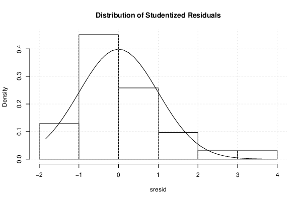
| Histogram | Compute |
| Central Tendency | Compute |
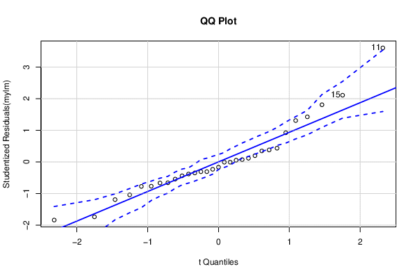
| QQ Plot | Compute |
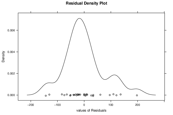
| Kernel Density Plot | Compute |
| Skewness/Kurtosis Test | Compute |
| Skewness-Kurtosis Plot | Compute |
| Harrell-Davis Plot | Compute |
| Bootstrap Plot -- Central Tendency | Compute |
| Blocked Bootstrap Plot -- Central Tendency | Compute |
| (Partial) Autocorrelation Plot | Compute |
| Spectral Analysis | Compute |
| Tukey lambda PPCC Plot | Compute |
| Box-Cox Normality Plot | Compute |
| Summary Statistics | Compute |
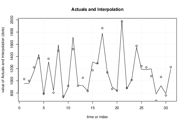
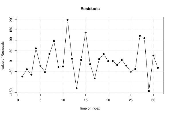
| Multiple Linear Regression - Actuals, Interpolation, and Residuals | |||
| Time or Index | Actuals | Interpolation Forecast | Residuals Prediction Error |
| 1 | 955 | 1029 | -74.23 |
| 2 | 960 | 999.8 | -39.81 |
| 3 | 1156 | 1221 | -65.05 |
| 4 | 1433 | 1372 | 60.53 |
| 5 | 769 | 791.6 | -22.59 |
| 6 | 1310 | 1362 | -52.32 |
| 7 | 840 | 806.1 | 33.85 |
| 8 | 1590 | 1494 | 95.78 |
| 9 | 716 | 744.8 | -28.82 |
| 10 | 892 | 918.1 | -26.06 |
| 11 | 1717 | 1520 | 197.5 |
| 12 | 930 | 918.7 | 11.26 |
| 13 | 920 | 1050 | -130.5 |
| 14 | 838 | 832.7 | 5.343 |
| 15 | 1310 | 1174 | 136.4 |
| 16 | 1275 | 1290 | -14.96 |
| 17 | 1780 | 1863 | -83.49 |
| 18 | 1148 | 1139 | 9.373 |
| 19 | 900 | 866.6 | 33.41 |
| 20 | 839 | 839.5 | -0.5395 |
| 21 | 1975 | 1975 | -0.07729 |
| 22 | 865 | 883.8 | -18.77 |
| 23 | 1018 | 1013 | 4.839 |
| 24 | 1550 | 1572 | -21.96 |
| 25 | 1190 | 1241 | -51.07 |
| 26 | 1182 | 1220 | -38.49 |
| 27 | 1198 | 1077 | 120.7 |
| 28 | 783 | 673.5 | 109.5 |
| 29 | 920 | 1064 | -143.8 |
| 30 | 788 | 761.5 | 26.45 |
| 31 | 1193 | 1225 | -32.46 |
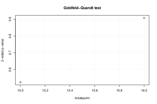
| Goldfeld-Quandt test for Heteroskedasticity | |||
| p-values | Alternative Hypothesis | ||
| breakpoint index | greater | 2-sided | less |
| 15 | 0.7382 | 0.5236 | 0.2618 |
| 16 | 0.5462 | 0.9077 | 0.4538 |
| Meta Analysis of Goldfeld-Quandt test for Heteroskedasticity | |||
| Description | # significant tests | % significant tests | OK/NOK |
| 1% type I error level | 0 | 0 | OK |
| 5% type I error level | 0 | 0 | OK |
| 10% type I error level | 0 | 0 | OK |
| Ramsey RESET F-Test for powers (2 and 3) of fitted values |
> reset_test_fitted RESET test data: mylm RESET = 4.7689, df1 = 2, df2 = 17, p-value = 0.0227 |
| Ramsey RESET F-Test for powers (2 and 3) of regressors |
> reset_test_regressors RESET test data: mylm RESET = -0.67407, df1 = 22, df2 = -3, p-value = NA |
| Ramsey RESET F-Test for powers (2 and 3) of principal components |
> reset_test_principal_components RESET test data: mylm RESET = 0.28945, df1 = 2, df2 = 17, p-value = 0.7523 |
| Variance Inflation Factors (Multicollinearity) |
> vif
        V        SQ       SQ2        BR        PH        GR        AG        Re
 1.390485 33.025181 23.863303  2.130852  1.563528  2.027583  7.275371  2.419217
        C        TH         T
 3.190228  3.048479  2.726906
|