| Multiple Linear Regression - Estimated Regression Equation |
| SP[t] = -440.624 + 117.332V[t] + 1.50169SQ[t] -0.000203676SQ2[t] + 41.4766BR[t] -65.1306PH[t] + 28.3809GR[t] -10.3153AG[t] + 115.739C[t] -262.201TH[t] + e[t] |
| Multiple Linear Regression - Ordinary Least Squares | |||||
| Variable | Parameter | S.D. | T-STAT H0: parameter = 0 | 2-tail p-value | 1-tail p-value |
| (Intercept) | -440.6 | 131.8 | -3.3440e+00 | 0.003076 | 0.001538 |
| V | +117.3 | 51.48 | +2.2790e+00 | 0.03321 | 0.01661 |
| SQ | +1.502 | 0.1498 | +1.0030e+01 | 1.848e-09 | 9.24e-10 |
| SQ2 | -0.0002037 | 2.9e-05 | -7.0240e+00 | 6.21e-07 | 3.105e-07 |
| BR | +41.48 | 41.62 | +9.9650e-01 | 0.3304 | 0.1652 |
| PH | -65.13 | 51.45 | -1.2660e+00 | 0.2194 | 0.1097 |
| GR | +28.38 | 57.48 | +4.9380e-01 | 0.6266 | 0.3133 |
| AG | -10.31 | 3.007 | -3.4300e+00 | 0.002513 | 0.001257 |
| C | +115.7 | 47.33 | +2.4450e+00 | 0.02337 | 0.01169 |
| TH | -262.2 | 79.22 | -3.3100e+00 | 0.003331 | 0.001666 |
| Multiple Linear Regression - Regression Statistics | |
| Multiple R | 0.9736 |
| R-squared | 0.9478 |
| Adjusted R-squared | 0.9255 |
| F-TEST (value) | 42.39 |
| F-TEST (DF numerator) | 9 |
| F-TEST (DF denominator) | 21 |
| p-value | 1.814e-11 |
| Multiple Linear Regression - Residual Statistics | |
| Residual Standard Deviation | 89.66 |
| Sum Squared Residuals | 1.688e+05 |
| Menu of Residual Diagnostics | |
| Description | Link |
| Histogram | Compute |
| Central Tendency | Compute |
| QQ Plot | Compute |
| Kernel Density Plot | Compute |
| Skewness/Kurtosis Test | Compute |
| Skewness-Kurtosis Plot | Compute |
| Harrell-Davis Plot | Compute |
| Bootstrap Plot -- Central Tendency | Compute |
| Blocked Bootstrap Plot -- Central Tendency | Compute |
| (Partial) Autocorrelation Plot | Compute |
| Spectral Analysis | Compute |
| Tukey lambda PPCC Plot | Compute |
| Box-Cox Normality Plot | Compute |
| Summary Statistics | Compute |
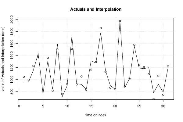
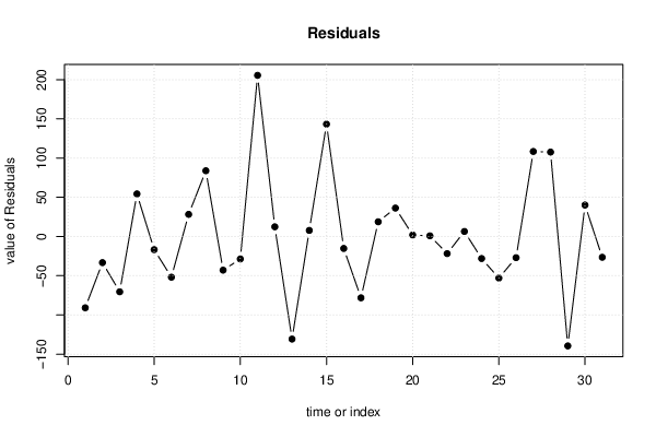
| Multiple Linear Regression - Actuals, Interpolation, and Residuals | |||
| Time or Index | Actuals | Interpolation Forecast | Residuals Prediction Error |
| 1 | 955 | 1046 | -90.95 |
| 2 | 960 | 993.3 | -33.31 |
| 3 | 1156 | 1227 | -70.51 |
| 4 | 1433 | 1379 | 54.28 |
| 5 | 769 | 785.8 | -16.79 |
| 6 | 1310 | 1362 | -51.89 |
| 7 | 840 | 811.8 | 28.21 |
| 8 | 1590 | 1506 | 83.83 |
| 9 | 716 | 758.9 | -42.95 |
| 10 | 892 | 920.7 | -28.69 |
| 11 | 1717 | 1512 | 205.5 |
| 12 | 930 | 917.6 | 12.35 |
| 13 | 920 | 1051 | -130.8 |
| 14 | 838 | 830.3 | 7.725 |
| 15 | 1310 | 1167 | 143.3 |
| 16 | 1275 | 1290 | -15.24 |
| 17 | 1780 | 1858 | -78.2 |
| 18 | 1148 | 1129 | 18.75 |
| 19 | 900 | 863.8 | 36.23 |
| 20 | 839 | 837.1 | 1.916 |
| 21 | 1975 | 1974 | 0.8799 |
| 22 | 865 | 886.8 | -21.85 |
| 23 | 1018 | 1012 | 6.414 |
| 24 | 1550 | 1578 | -28.15 |
| 25 | 1190 | 1243 | -53 |
| 26 | 1182 | 1209 | -27.01 |
| 27 | 1198 | 1090 | 108.4 |
| 28 | 783 | 675.4 | 107.6 |
| 29 | 920 | 1060 | -139.6 |
| 30 | 788 | 747.9 | 40.1 |
| 31 | 1193 | 1220 | -26.52 |
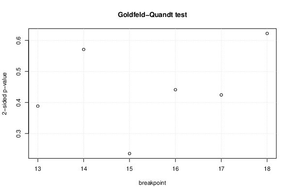
| Goldfeld-Quandt test for Heteroskedasticity | |||
| p-values | Alternative Hypothesis | ||
| breakpoint index | greater | 2-sided | less |
| 13 | 0.8058 | 0.3883 | 0.1942 |
| 14 | 0.7146 | 0.5709 | 0.2854 |
| 15 | 0.8823 | 0.2353 | 0.1177 |
| 16 | 0.7795 | 0.4411 | 0.2205 |
| 17 | 0.7878 | 0.4243 | 0.2122 |
| 18 | 0.6888 | 0.6224 | 0.3112 |
| Meta Analysis of Goldfeld-Quandt test for Heteroskedasticity | |||
| Description | # significant tests | % significant tests | OK/NOK |
| 1% type I error level | 0 | 0 | OK |
| 5% type I error level | 0 | 0 | OK |
| 10% type I error level | 0 | 0 | OK |
| Ramsey RESET F-Test for powers (2 and 3) of fitted values |
> reset_test_fitted RESET test data: mylm RESET = 4.4882, df1 = 2, df2 = 19, p-value = 0.02533 |
| Ramsey RESET F-Test for powers (2 and 3) of regressors |
> reset_test_regressors RESET test data: mylm RESET = 0.14002, df1 = 18, df2 = 3, p-value = 0.9977 |
| Ramsey RESET F-Test for powers (2 and 3) of principal components |
> reset_test_principal_components RESET test data: mylm RESET = 0.40167, df1 = 2, df2 = 19, p-value = 0.6748 |
| Variance Inflation Factors (Multicollinearity) |
> vif
        V        SQ       SQ2        BR        PH        GR        AG         C
 1.367309 31.692274 23.416246  2.057855  1.380795  1.431832  2.739743  2.157496
       TH
 2.719387
|