| Multiple Linear Regression - Estimated Regression Equation |
| DPSF[t] = + 0.949905 + 0.140787V[t] -0.000148272SQ[t] -4.32454e-09SQ2[t] + 0.0415811BR[t] + e[t] |
| Multiple Linear Regression - Ordinary Least Squares | |||||
| Variable | Parameter | S.D. | T-STAT H0: parameter = 0 | 2-tail p-value | 1-tail p-value |
| (Intercept) | +0.9499 | 0.1842 | +5.1580e+00 | 2.218e-05 | 1.109e-05 |
| V | +0.1408 | 0.06824 | +2.0630e+00 | 0.04921 | 0.02461 |
| SQ | -0.0001483 | 0.0001702 | -8.7110e-01 | 0.3917 | 0.1958 |
| SQ2 | -4.325e-09 | 3.821e-08 | -1.1320e-01 | 0.9108 | 0.4554 |
| BR | +0.04158 | 0.05523 | +7.5290e-01 | 0.4582 | 0.2291 |
| Multiple Linear Regression - Regression Statistics | |
| Multiple R | 0.6751 |
| R-squared | 0.4557 |
| Adjusted R-squared | 0.372 |
| F-TEST (value) | 5.443 |
| F-TEST (DF numerator) | 4 |
| F-TEST (DF denominator) | 26 |
| p-value | 0.002546 |
| Multiple Linear Regression - Residual Statistics | |
| Residual Standard Deviation | 0.1348 |
| Sum Squared Residuals | 0.4727 |
| Menu of Residual Diagnostics | |
| Description | Link |
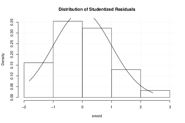
| Histogram | Compute |
| Central Tendency | Compute |
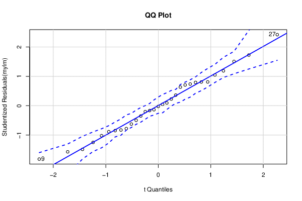
| QQ Plot | Compute |
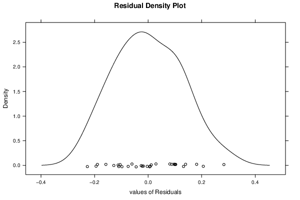
| Kernel Density Plot | Compute |
| Skewness/Kurtosis Test | Compute |
| Skewness-Kurtosis Plot | Compute |
| Harrell-Davis Plot | Compute |
| Bootstrap Plot -- Central Tendency | Compute |
| Blocked Bootstrap Plot -- Central Tendency | Compute |
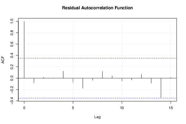
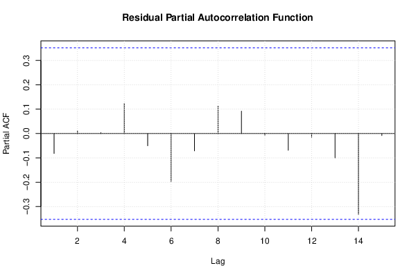
| (Partial) Autocorrelation Plot | Compute |
| Spectral Analysis | Compute |
| Tukey lambda PPCC Plot | Compute |
| Box-Cox Normality Plot | Compute |
| Summary Statistics | Compute |
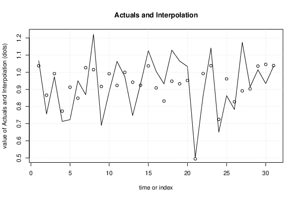
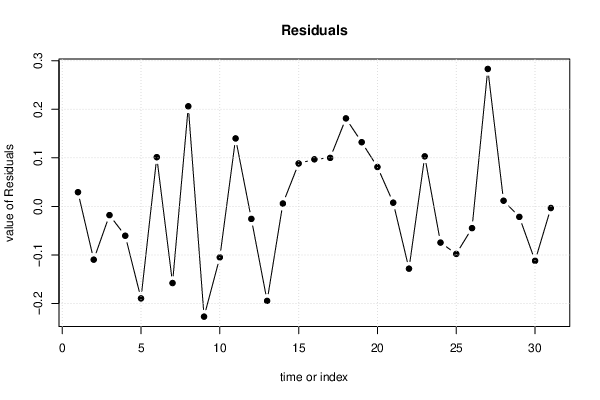
| Multiple Linear Regression - Actuals, Interpolation, and Residuals | |||
| Time or Index | Actuals | Interpolation Forecast | Residuals Prediction Error |
| 1 | 1.067 | 1.038 | 0.02935 |
| 2 | 0.7565 | 0.8661 | -0.1096 |
| 3 | 0.9739 | 0.9918 | -0.01788 |
| 4 | 0.7129 | 0.7732 | -0.06029 |
| 5 | 0.7234 | 0.9128 | -0.1894 |
| 6 | 0.95 | 0.8485 | 0.1014 |
| 7 | 0.8687 | 1.026 | -0.1578 |
| 8 | 1.221 | 1.015 | 0.2061 |
| 9 | 0.6898 | 0.9167 | -0.2269 |
| 10 | 0.8867 | 0.9915 | -0.1048 |
| 11 | 1.063 | 0.9231 | 0.14 |
| 12 | 0.9738 | 0.9995 | -0.02568 |
| 13 | 0.7474 | 0.9419 | -0.1945 |
| 14 | 0.9301 | 0.9241 | 0.005958 |
| 15 | 1.125 | 1.037 | 0.08844 |
| 16 | 1.006 | 0.9085 | 0.09702 |
| 17 | 0.9319 | 0.832 | 0.09995 |
| 18 | 1.129 | 0.9475 | 0.1813 |
| 19 | 1.065 | 0.9328 | 0.1322 |
| 20 | 1.033 | 0.9521 | 0.0812 |
| 21 | 0.5024 | 0.4947 | 0.007715 |
| 22 | 0.8641 | 0.9923 | -0.1282 |
| 23 | 1.141 | 1.038 | 0.1031 |
| 24 | 0.6504 | 0.7249 | -0.07447 |
| 25 | 0.8636 | 0.9613 | -0.09775 |
| 26 | 0.7828 | 0.8275 | -0.04469 |
| 27 | 1.175 | 0.8914 | 0.2831 |
| 28 | 0.9147 | 0.903 | 0.01174 |
| 29 | 1.014 | 1.036 | -0.02148 |
| 30 | 0.9336 | 1.046 | -0.112 |
| 31 | 1.036 | 1.039 | -0.003296 |
| Goldfeld-Quandt test for Heteroskedasticity | |||
| p-values | Alternative Hypothesis | ||
| breakpoint index | greater | 2-sided | less |
| 8 | 0.6084 | 0.7833 | 0.3916 |
| 9 | 0.6002 | 0.7996 | 0.3998 |
| 10 | 0.4637 | 0.9274 | 0.5363 |
| 11 | 0.3717 | 0.7433 | 0.6283 |
| 12 | 0.2854 | 0.5707 | 0.7146 |
| 13 | 0.5622 | 0.8757 | 0.4378 |
| 14 | 0.6701 | 0.6598 | 0.3299 |
| 15 | 0.6035 | 0.793 | 0.3965 |
| 16 | 0.5525 | 0.8949 | 0.4475 |
| 17 | 0.5209 | 0.9583 | 0.4791 |
| 18 | 0.6886 | 0.6229 | 0.3114 |
| 19 | 0.6862 | 0.6276 | 0.3138 |
| 20 | 0.5779 | 0.8442 | 0.4221 |
| 21 | 0.4375 | 0.8751 | 0.5625 |
| 22 | 0.4395 | 0.8791 | 0.5605 |
| 23 | 0.4147 | 0.8293 | 0.5853 |
| Meta Analysis of Goldfeld-Quandt test for Heteroskedasticity | |||
| Description | # significant tests | % significant tests | OK/NOK |
| 1% type I error level | 0 | 0 | OK |
| 5% type I error level | 0 | 0 | OK |
| 10% type I error level | 0 | 0 | OK |
| Ramsey RESET F-Test for powers (2 and 3) of fitted values |
> reset_test_fitted RESET test data: mylm RESET = 0.30979, df1 = 2, df2 = 24, p-value = 0.7365 |
| Ramsey RESET F-Test for powers (2 and 3) of regressors |
> reset_test_regressors RESET test data: mylm RESET = 0.6392, df1 = 8, df2 = 18, p-value = 0.7354 |
| Ramsey RESET F-Test for powers (2 and 3) of principal components |
> reset_test_principal_components RESET test data: mylm RESET = 0.72839, df1 = 2, df2 = 24, p-value = 0.4931 |
| Variance Inflation Factors (Multicollinearity) |
> vif
        V        SQ       SQ2        BR
 1.062316 18.103205 17.978076  1.601784
|