| Multiple Linear Regression - Estimated Regression Equation |
| DPSF[t] = + 0.791453 + 0.0936654V[t] + 0.000129461SQ[t] -3.72685e-08SQ2[t] + 0.0349066BR[t] -0.0441961PH[t] + 0.031338GR[t] -0.00971863AG[t] + 0.0964604C[t] -0.121352TH[t] + e[t] |
| Multiple Linear Regression - Ordinary Least Squares | |||||
| Variable | Parameter | S.D. | T-STAT H0: parameter = 0 | 2-tail p-value | 1-tail p-value |
| (Intercept) | +0.7914 | 0.1091 | +7.2540e+00 | 3.809e-07 | 1.904e-07 |
| V | +0.09366 | 0.04263 | +2.1970e+00 | 0.03935 | 0.01967 |
| SQ | +0.0001295 | 0.000124 | +1.0440e+00 | 0.3084 | 0.1542 |
| SQ2 | -3.727e-08 | 2.401e-08 | -1.5520e+00 | 0.1356 | 0.06778 |
| BR | +0.03491 | 0.03447 | +1.0130e+00 | 0.3227 | 0.1613 |
| PH | -0.0442 | 0.0426 | -1.0370e+00 | 0.3113 | 0.1557 |
| GR | +0.03134 | 0.04759 | +6.5840e-01 | 0.5174 | 0.2587 |
| AG | -0.009719 | 0.00249 | -3.9030e+00 | 0.0008189 | 0.0004095 |
| C | +0.09646 | 0.03919 | +2.4610e+00 | 0.02259 | 0.01129 |
| TH | -0.1213 | 0.06559 | -1.8500e+00 | 0.07842 | 0.03921 |
| Multiple Linear Regression - Regression Statistics | |
| Multiple R | 0.931 |
| R-squared | 0.8667 |
| Adjusted R-squared | 0.8096 |
| F-TEST (value) | 15.18 |
| F-TEST (DF numerator) | 9 |
| F-TEST (DF denominator) | 21 |
| p-value | 2.582e-07 |
| Multiple Linear Regression - Residual Statistics | |
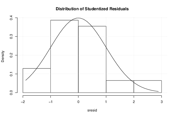
| Residual Standard Deviation | 0.07424 |
| Sum Squared Residuals | 0.1157 |
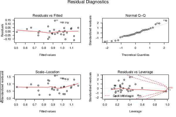
| Menu of Residual Diagnostics | |
| Description | Link |
| Histogram | Compute |
| Central Tendency | Compute |
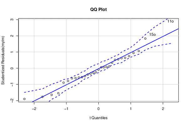
| QQ Plot | Compute |
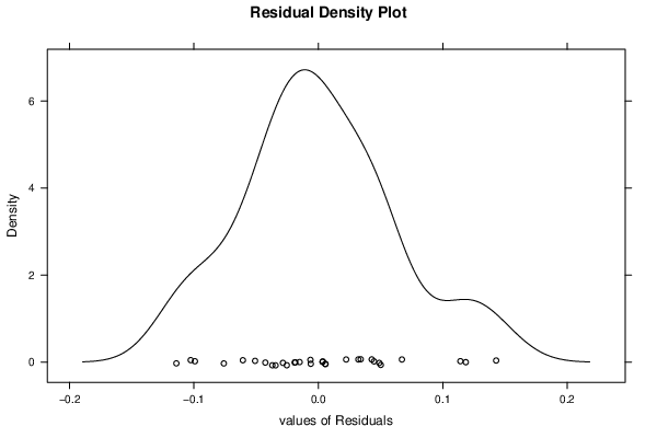
| Kernel Density Plot | Compute |
| Skewness/Kurtosis Test | Compute |
| Skewness-Kurtosis Plot | Compute |
| Harrell-Davis Plot | Compute |
| Bootstrap Plot -- Central Tendency | Compute |
| Blocked Bootstrap Plot -- Central Tendency | Compute |
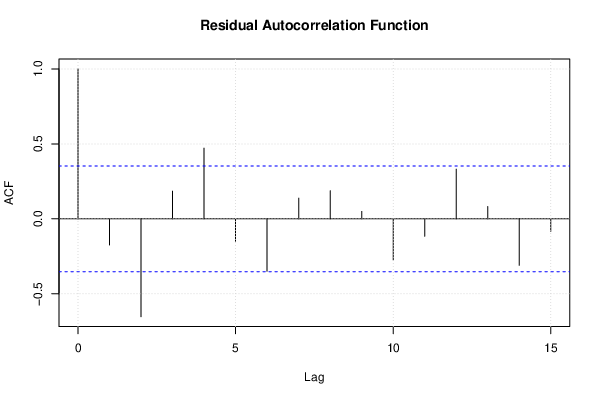
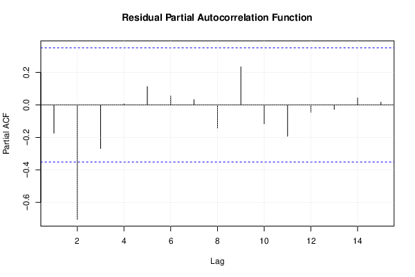
| (Partial) Autocorrelation Plot | Compute |
| Spectral Analysis | Compute |
| Tukey lambda PPCC Plot | Compute |
| Box-Cox Normality Plot | Compute |
| Summary Statistics | Compute |
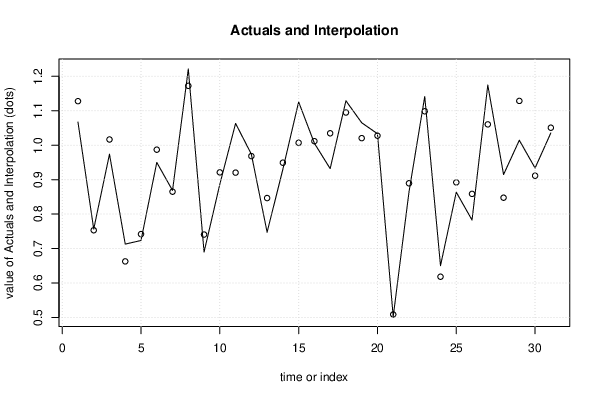
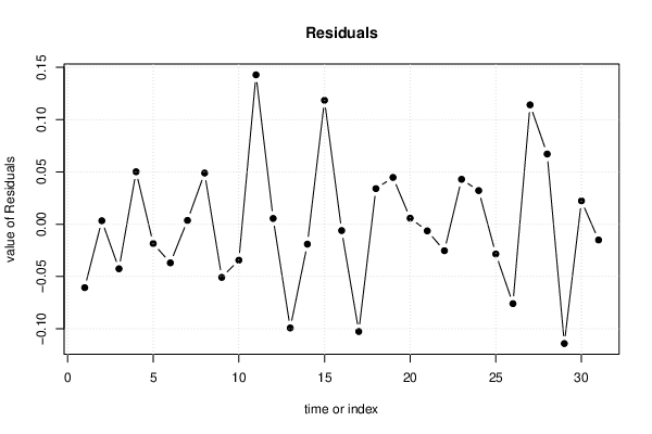
| Multiple Linear Regression - Actuals, Interpolation, and Residuals | |||
| Time or Index | Actuals | Interpolation Forecast | Residuals Prediction Error |
| 1 | 1.067 | 1.128 | -0.06065 |
| 2 | 0.7565 | 0.7532 | 0.003297 |
| 3 | 0.9739 | 1.016 | -0.04261 |
| 4 | 0.7129 | 0.6628 | 0.05016 |
| 5 | 0.7234 | 0.7419 | -0.01848 |
| 6 | 0.95 | 0.9869 | -0.03697 |
| 7 | 0.8687 | 0.865 | 0.003652 |
| 8 | 1.221 | 1.172 | 0.04896 |
| 9 | 0.6898 | 0.7406 | -0.05084 |
| 10 | 0.8867 | 0.9211 | -0.0344 |
| 11 | 1.063 | 0.9203 | 0.1429 |
| 12 | 0.9738 | 0.9683 | 0.00553 |
| 13 | 0.7474 | 0.8466 | -0.09919 |
| 14 | 0.9301 | 0.9491 | -0.01906 |
| 15 | 1.125 | 1.007 | 0.1185 |
| 16 | 1.006 | 1.012 | -0.006088 |
| 17 | 0.9319 | 1.035 | -0.1026 |
| 18 | 1.129 | 1.095 | 0.03405 |
| 19 | 1.065 | 1.02 | 0.04472 |
| 20 | 1.033 | 1.028 | 0.00575 |
| 21 | 0.5024 | 0.5088 | -0.006371 |
| 22 | 0.8641 | 0.8895 | -0.02534 |
| 23 | 1.141 | 1.098 | 0.04291 |
| 24 | 0.6504 | 0.6183 | 0.03214 |
| 25 | 0.8636 | 0.892 | -0.02845 |
| 26 | 0.7828 | 0.8587 | -0.07593 |
| 27 | 1.175 | 1.06 | 0.1141 |
| 28 | 0.9147 | 0.8476 | 0.06713 |
| 29 | 1.014 | 1.128 | -0.1141 |
| 30 | 0.9336 | 0.9113 | 0.02234 |
| 31 | 1.036 | 1.051 | -0.01505 |
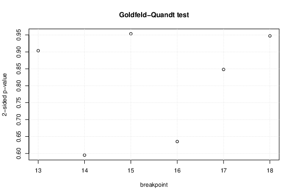
| Goldfeld-Quandt test for Heteroskedasticity | |||
| p-values | Alternative Hypothesis | ||
| breakpoint index | greater | 2-sided | less |
| 13 | 0.4517 | 0.9034 | 0.5483 |
| 14 | 0.2975 | 0.5949 | 0.7025 |
| 15 | 0.4767 | 0.9535 | 0.5233 |
| 16 | 0.3176 | 0.6352 | 0.6824 |
| 17 | 0.5759 | 0.8481 | 0.4241 |
| 18 | 0.5264 | 0.9472 | 0.4736 |
| Meta Analysis of Goldfeld-Quandt test for Heteroskedasticity | |||
| Description | # significant tests | % significant tests | OK/NOK |
| 1% type I error level | 0 | 0 | OK |
| 5% type I error level | 0 | 0 | OK |
| 10% type I error level | 0 | 0 | OK |
| Ramsey RESET F-Test for powers (2 and 3) of fitted values |
> reset_test_fitted RESET test data: mylm RESET = 0.64126, df1 = 2, df2 = 19, p-value = 0.5376 |
| Ramsey RESET F-Test for powers (2 and 3) of regressors |
> reset_test_regressors RESET test data: mylm RESET = 0.15411, df1 = 18, df2 = 3, p-value = 0.9964 |
| Ramsey RESET F-Test for powers (2 and 3) of principal components |
> reset_test_principal_components RESET test data: mylm RESET = 0.17358, df1 = 2, df2 = 19, p-value = 0.842 |
| Variance Inflation Factors (Multicollinearity) |
> vif
        V        SQ       SQ2        BR        PH        GR        AG         C
 1.367309 31.692274 23.416246  2.057855  1.380795  1.431832  2.739743  2.157496
       TH
 2.719387
|