Free Statistics

of Irreproducible Research!

Author's title

Author*The author of this computation has been verified*
R Software Modulerwasp_Tests to Compare Two Means.wasp
Title produced by softwareT-Tests
Date of computationSat, 16 Oct 2021 22:30:31 +0200
Cite this page as followsStatistical Computations at FreeStatistics.org, Office for Research Development and Education, URL https://freestatistics.org/blog/index.php?v=date/2021/Oct/16/t163441665694y33422ao0afag.htm/, Retrieved Fri, 19 Apr 2024 21:58:25 +0200
Statistical Computations at FreeStatistics.org, Office for Research Development and Education, URL https://freestatistics.org/blog/index.php?pk=, Retrieved Fri, 19 Apr 2024 21:58:25 +0200
QR Codes:

Original text written by user:"How likely are you to a plant a tree in the future?" by "Colloquiuum class? Yes or No."
IsPrivate?This computation is private
User-defined keywords
Estimated Impact0
Dataseries X:
19	4
15	0
14	1
3	0
0	0


Summary of computational transaction
Raw Input view raw input (R code)
Raw Outputview raw output of R engine
Computing time0 seconds
R ServerBig Analytics Cloud Computing Center

\begin{tabular}{lllllllll}
\hline
Summary of computational transaction \tabularnewline
Raw Input view raw input (R code)  \tabularnewline
Raw Outputview raw output of R engine  \tabularnewline
Computing time0 seconds \tabularnewline
R ServerBig Analytics Cloud Computing Center \tabularnewline
\hline
\end{tabular}
%Source: https://freestatistics.org/blog/index.php?pk=&T=0

[TABLE]
[ROW]
Summary of computational transaction[/C][/ROW] [ROW]Raw Input[/C] view raw input (R code) [/C][/ROW] [ROW]Raw Output[/C]view raw output of R engine [/C][/ROW] [ROW]Computing time[/C]0 seconds[/C][/ROW] [ROW]R Server[/C]Big Analytics Cloud Computing Center[/C][/ROW] [/TABLE] Source: https://freestatistics.org/blog/index.php?pk=&T=0

Globally Unique Identifier (entire table): ba.freestatistics.org/blog/index.php?pk=&T=0

As an alternative you can also use a QR Code:  

The GUIDs for individual cells are displayed in the table below:

Summary of computational transaction
Raw Input view raw input (R code)
Raw Outputview raw output of R engine
Computing time0 seconds
R ServerBig Analytics Cloud Computing Center


Wilcoxon Test
StatisticP-value
Wilcoxon Test20.50.106

\begin{tabular}{lllllllll}
\hline
Wilcoxon Test \tabularnewline
 & Statistic & P-value \tabularnewline
Wilcoxon Test & 20.5 & 0.106 \tabularnewline
\hline
\end{tabular}
%Source: https://freestatistics.org/blog/index.php?pk=&T=1

[TABLE]
[ROW][C]Wilcoxon Test[/C][/ROW]
[ROW][C][/C][C]Statistic[/C][C]P-value[/C][/ROW]
[ROW][C]Wilcoxon Test[/C][C]20.5[/C][C]0.106[/C][/ROW]
[/TABLE]
Source: https://freestatistics.org/blog/index.php?pk=&T=1

Globally Unique Identifier (entire table): ba.freestatistics.org/blog/index.php?pk=&T=1

As an alternative you can also use a QR Code:  

The GUIDs for individual cells are displayed in the table below:

Wilcoxon Test
StatisticP-value
Wilcoxon Test20.50.106


Standard Deviations
Variable 18.228
Variable 21.73205

\begin{tabular}{lllllllll}
\hline
Standard Deviations \tabularnewline
Variable 1 & 8.228 \tabularnewline
Variable 2 & 1.73205 \tabularnewline
\hline
\end{tabular}
%Source: https://freestatistics.org/blog/index.php?pk=&T=2

[TABLE]
[ROW][C]Standard Deviations[/C][/ROW]
[ROW][C]Variable 1[/C][C]8.228[/C][/ROW]
[ROW][C]Variable 2[/C][C]1.73205[/C][/ROW]
[/TABLE]
Source: https://freestatistics.org/blog/index.php?pk=&T=2

Globally Unique Identifier (entire table): ba.freestatistics.org/blog/index.php?pk=&T=2

As an alternative you can also use a QR Code:  

The GUIDs for individual cells are displayed in the table below:

Standard Deviations
Variable 18.228
Variable 21.73205


Parameters (Session):
par1 = two.sided ; par2 = 1 ; par3 = 2 ; par4 = Wilcoxon-Mann_Whitney ; par5 = unpaired ; par6 = 0.0 ; par7 = 0.95 ; par8 = TRUE ;
Parameters (R input):
par1 = two.sided ; par2 = 1 ; par3 = 2 ; par4 = Wilcoxon-Mann_Whitney ; par5 = unpaired ; par6 = 0.0 ; par7 = 0.95 ; par8 = TRUE ;
R code (references can be found in the software module):
par8 <- 'TRUE'
par7 <- '0.95'
par6 <- '0.0'
par5 <- 'unpaired'
par4 <- 'Wilcoxon-Mann_Whitney'
par3 <- '2'
par2 <- '1'
par1 <- 'two.sided'
par2 <- as.numeric(par2)
par3 <- as.numeric(par3)
par4 <- as.character(par4)
par5 <- as.character(par5)
par6 <- as.numeric(par6)
par7 <- as.numeric(par7)
par8 <- as.logical(par8)
if ( par5 == 'unpaired') paired <- FALSE else paired <- TRUE
x <- t(y)
if(par8){
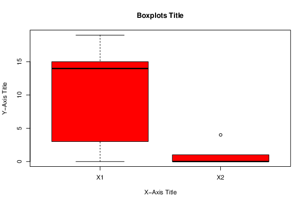
bitmap(file='test1.png')
(r<-boxplot(x ,xlab=xlab,ylab=ylab,main=main,notch=FALSE,col=2))
dev.off()
}
load(file='createtable')
if( par4 == 'Wilcoxon-Mann_Whitney'){
a<-table.start()
a <- table.row.start(a)
a <- table.element(a,'Wilcoxon Test',3,TRUE)
a <- table.row.end(a)
a <- table.row.start(a)
a <- table.element(a,'',1,TRUE)
a <- table.element(a,'Statistic',1,TRUE)
a <- table.element(a,'P-value',1,TRUE)
a <- table.row.end(a)
W <- wilcox.test(x[,par2],x[,par3],alternative=par1, paired = paired)
a<-table.row.start(a)
a<-table.element(a,'Wilcoxon Test',1,TRUE)
a<-table.element(a,W$statistic[[1]])
a<-table.element(a,round(W$p.value, digits=5) )
a<-table.row.end(a)
a<-table.end(a)
table.save(a,file='mytable.tab')
}
if( par4 == 'T-Test')
{
T <- t.test(x[,par2],x[,par3],alternative=par1, paired=paired, mu=par6, conf.level=par7)
a<-table.start()
a <- table.row.start(a)
a <- table.element(a,'T-Test',3,TRUE)
a <- table.row.end(a)
if(paired){
a <- table.row.start(a)
a <- table.element(a,'Difference: Mean1 - Mean2',1,TRUE)
a<-table.element(a,round(T$estimate, digits=5) )
a <- table.row.end(a)
}
if(!paired){
a <- table.row.start(a)
a <- table.element(a,'Mean1',1,TRUE)
a<-table.element(a,round(T$estimate[1], digits=5) )
a <- table.row.end(a)
a <- table.row.start(a)
a <- table.element(a,'Mean2',1,TRUE)
a<-table.element(a,round(T$estimate[2], digits=5) )
a <- table.row.end(a)
}
a <- table.row.start(a)
a <- table.element(a,'T Statistic',1,TRUE)
a<-table.element(a,round(T$statistic, digits=5) )
a <- table.row.end(a)
a <- table.row.start(a)
a <- table.element(a,'P-value',1,TRUE)
a<-table.element(a,round(T$p.value, digits=5) )
a <- table.row.end(a)
a <- table.row.start(a)
a <- table.element(a,'Lower Confidence Limit',1,TRUE)
a<-table.element(a,round(T$conf.int[1], digits=5) )
a <- table.row.end(a)
a<-table.row.start(a)
a <- table.element(a,'Upper Confidence Limit',1,TRUE)
a<-table.element(a,round(T$conf.int[2], digits=5) )
a <- table.row.end(a)
a<-table.end(a)
table.save(a,file='mytable.tab')
}
a<-table.start()
a <- table.row.start(a)
a <- table.element(a,'Standard Deviations',3,TRUE)
a <- table.row.end(a)
a <- table.row.start(a)
a <- table.element(a,'Variable 1',1,TRUE)
a<-table.element(a,round(sd(x[,par2], na.rm=TRUE), digits=5) )
a <- table.row.end(a)
a <- table.row.start(a)
a <- table.element(a,'Variable 2',1,TRUE)
a<-table.element(a,round(sd(x[,par3], na.rm=TRUE), digits=5) )
a <- table.row.end(a)
a<-table.end(a)
table.save(a,file='mytable1.tab')