Free Statistics
of Irreproducible Research!
Description of Statistical Computation | |||||||||||||||||||||
|---|---|---|---|---|---|---|---|---|---|---|---|---|---|---|---|---|---|---|---|---|---|
| Author's title | |||||||||||||||||||||
| Author | *Unverified author* | ||||||||||||||||||||
| R Software Module | rwasp_meanplot.wasp | ||||||||||||||||||||
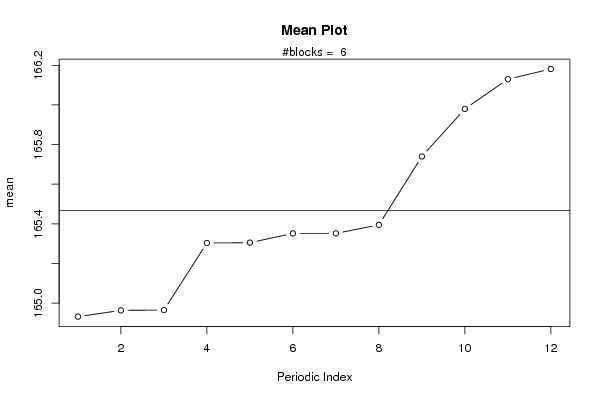
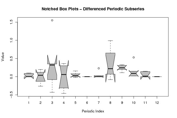
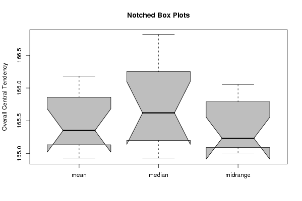
| Title produced by software | Mean Plot | ||||||||||||||||||||
| Date of computation | Tue, 22 Apr 2008 06:40:21 -0600 | ||||||||||||||||||||
| Cite this page as follows | Statistical Computations at FreeStatistics.org, Office for Research Development and Education, URL https://freestatistics.org/blog/index.php?v=date/2008/Apr/22/t1208868084heikzmakv431v8q.htm/, Retrieved Mon, 13 May 2024 20:03:01 +0000 | ||||||||||||||||||||
| Statistical Computations at FreeStatistics.org, Office for Research Development and Education, URL https://freestatistics.org/blog/index.php?pk=10626, Retrieved Mon, 13 May 2024 20:03:01 +0000 | |||||||||||||||||||||
| QR Codes: | |||||||||||||||||||||
|
| |||||||||||||||||||||
| Original text written by user: | |||||||||||||||||||||
| IsPrivate? | No (this computation is public) | ||||||||||||||||||||
| User-defined keywords | |||||||||||||||||||||
| Estimated Impact | 262 | ||||||||||||||||||||
Tree of Dependent Computations | |||||||||||||||||||||
| Family? (F = Feedback message, R = changed R code, M = changed R Module, P = changed Parameters, D = changed Data) | |||||||||||||||||||||
| - [Mean Plot] [Mean Plot - Blaze...] [2008-04-22 12:40:21] [18a9c7462de321e50920adc850709d38] [Current] | |||||||||||||||||||||
| Feedback Forum | |||||||||||||||||||||
Post a new message | |||||||||||||||||||||
Dataset | |||||||||||||||||||||
| Dataseries X: | |||||||||||||||||||||
161,79 161,79 161,85 161,77 161,86 161,89 161,89 161,89 162,18 162,43 162,58 162,57 162,57 162,57 162,44 162,79 163,15 163,23 163,23 163,23 163,38 163,71 163,73 163,73 163,73 163,73 163,93 164,27 164,57 164,73 164,73 164,76 165,75 165,86 165,99 166,13 166,13 166,13 166,15 166,45 166,48 166,51 166,51 166,51 166,58 166,82 167,35 167,5 167,5 167,6 167,72 167,29 166,98 166,98 166,98 166,98 167,63 167,83 167,85 167,87 167,87 167,96 167,7 169,25 168,79 168,77 168,77 169 168,92 169,23 169,28 169,29 | |||||||||||||||||||||
Tables (Output of Computation) | |||||||||||||||||||||
| |||||||||||||||||||||
Figures (Output of Computation) | |||||||||||||||||||||
Input Parameters & R Code | |||||||||||||||||||||
| Parameters (Session): | |||||||||||||||||||||
| par1 = 12 ; | |||||||||||||||||||||
| Parameters (R input): | |||||||||||||||||||||
| par1 = 12 ; | |||||||||||||||||||||
| R code (references can be found in the software module): | |||||||||||||||||||||
par1 <- as.numeric(par1) | |||||||||||||||||||||