Free Statistics
of Irreproducible Research!
Description of Statistical Computation | |||||||||||||||||||||
|---|---|---|---|---|---|---|---|---|---|---|---|---|---|---|---|---|---|---|---|---|---|
| Author's title | |||||||||||||||||||||
| Author | *Unverified author* | ||||||||||||||||||||
| R Software Module | rwasp_meanplot.wasp | ||||||||||||||||||||
| Title produced by software | Mean Plot | ||||||||||||||||||||
| Date of computation | Tue, 22 Apr 2008 13:42:21 -0600 | ||||||||||||||||||||
| Cite this page as follows | Statistical Computations at FreeStatistics.org, Office for Research Development and Education, URL https://freestatistics.org/blog/index.php?v=date/2008/Apr/22/t1208893424n7ycr2gf0eqp549.htm/, Retrieved Sun, 12 May 2024 14:25:21 +0000 | ||||||||||||||||||||
| Statistical Computations at FreeStatistics.org, Office for Research Development and Education, URL https://freestatistics.org/blog/index.php?pk=10646, Retrieved Sun, 12 May 2024 14:25:21 +0000 | |||||||||||||||||||||
| QR Codes: | |||||||||||||||||||||
|
| |||||||||||||||||||||
| Original text written by user: | |||||||||||||||||||||
| IsPrivate? | No (this computation is public) | ||||||||||||||||||||
| User-defined keywords | |||||||||||||||||||||
| Estimated Impact | 144 | ||||||||||||||||||||
Tree of Dependent Computations | |||||||||||||||||||||
| Family? (F = Feedback message, R = changed R code, M = changed R Module, P = changed Parameters, D = changed Data) | |||||||||||||||||||||
| - [Mean Plot] [Mean Plot - maan...] [2008-04-22 19:42:21] [10bf337d6aaebcf0c700ebf73b3b2ad5] [Current] | |||||||||||||||||||||
| Feedback Forum | |||||||||||||||||||||
Post a new message | |||||||||||||||||||||
Dataset | |||||||||||||||||||||
| Dataseries X: | |||||||||||||||||||||
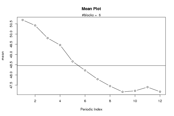
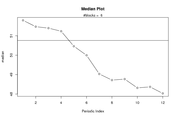
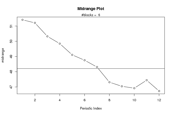
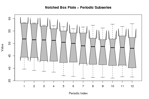
58,1 57,9 57,3 55,9 55 55,9 56,6 57,3 56,2 57,7 56,8 57,9 58,3 58,2 56,9 57,1 56,7 54,2 54,2 52,1 51,5 51,8 53 52,4 52,41 52,36 52,94 52,34 51,84 51,42 50,85 50,66 51,53 51,59 52,32 51,98 51,17 50,57 49,84 50,12 49,08 48,57 47,22 46,78 46,04 45,05 44,42 44,09 44,46 44,34 43,04 42,87 42,32 42,49 41,94 41,6 41,42 41,12 41,28 40,21 39,69 39,16 38,8 38,44 37,02 36,75 35,95 36,29 36,35 36,07 36,6 36,5 | |||||||||||||||||||||
Tables (Output of Computation) | |||||||||||||||||||||
| |||||||||||||||||||||
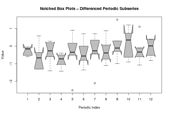
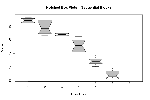
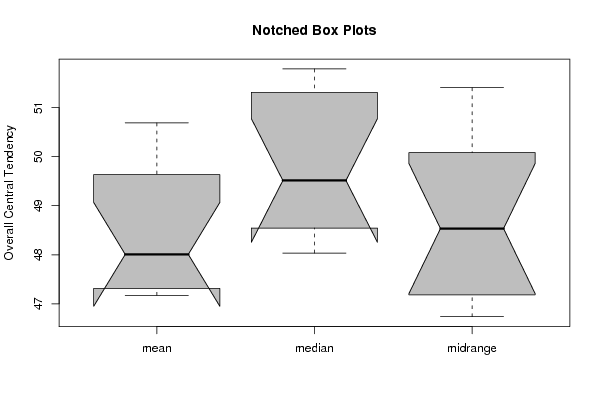
Figures (Output of Computation) | |||||||||||||||||||||
Input Parameters & R Code | |||||||||||||||||||||
| Parameters (Session): | |||||||||||||||||||||
| par1 = 12 ; | |||||||||||||||||||||
| Parameters (R input): | |||||||||||||||||||||
| par1 = 12 ; | |||||||||||||||||||||
| R code (references can be found in the software module): | |||||||||||||||||||||
par1 <- as.numeric(par1) | |||||||||||||||||||||