Free Statistics
of Irreproducible Research!
Description of Statistical Computation | |||||||||||||||||||||
|---|---|---|---|---|---|---|---|---|---|---|---|---|---|---|---|---|---|---|---|---|---|
| Author's title | |||||||||||||||||||||
| Author | *Unverified author* | ||||||||||||||||||||
| R Software Module | rwasp_meanplot.wasp | ||||||||||||||||||||
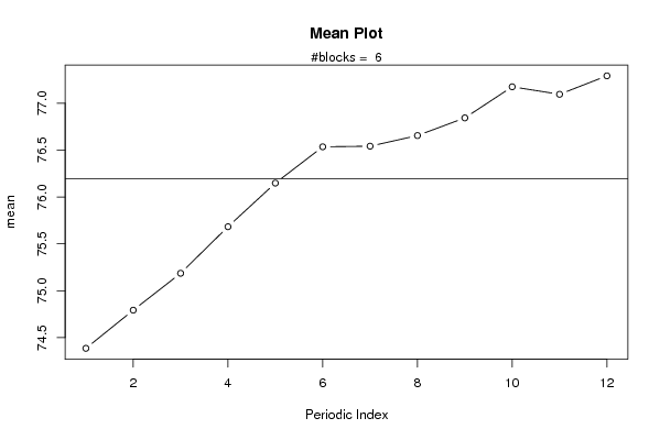
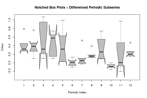
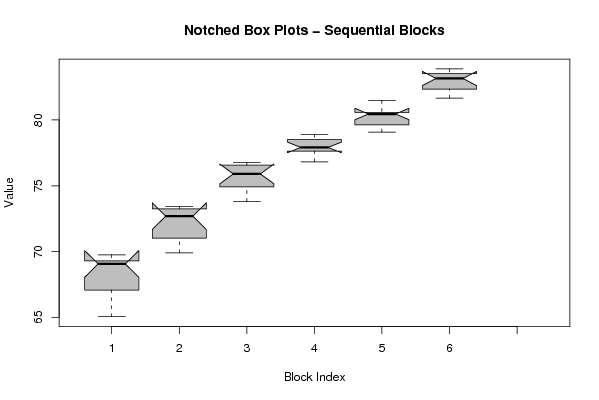
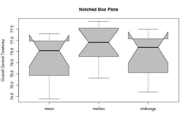
| Title produced by software | Mean Plot | ||||||||||||||||||||
| Date of computation | Sat, 26 Apr 2008 10:09:20 -0600 | ||||||||||||||||||||
| Cite this page as follows | Statistical Computations at FreeStatistics.org, Office for Research Development and Education, URL https://freestatistics.org/blog/index.php?v=date/2008/Apr/26/t12092262089fpj844tfs9nddk.htm/, Retrieved Sun, 12 May 2024 18:19:54 +0000 | ||||||||||||||||||||
| Statistical Computations at FreeStatistics.org, Office for Research Development and Education, URL https://freestatistics.org/blog/index.php?pk=10743, Retrieved Sun, 12 May 2024 18:19:54 +0000 | |||||||||||||||||||||
| QR Codes: | |||||||||||||||||||||
|
| |||||||||||||||||||||
| Original text written by user: | |||||||||||||||||||||
| IsPrivate? | No (this computation is public) | ||||||||||||||||||||
| User-defined keywords | |||||||||||||||||||||
| Estimated Impact | 253 | ||||||||||||||||||||
Tree of Dependent Computations | |||||||||||||||||||||
| Family? (F = Feedback message, R = changed R code, M = changed R Module, P = changed Parameters, D = changed Data) | |||||||||||||||||||||
| - [Mean Plot] [Michiel van Schai...] [2008-04-26 16:09:20] [f1389fff7fe55b9c206fc4c1b90cd78e] [Current] | |||||||||||||||||||||
| Feedback Forum | |||||||||||||||||||||
Post a new message | |||||||||||||||||||||
Dataset | |||||||||||||||||||||
| Dataseries X: | |||||||||||||||||||||
65,05 65,84 66,6 67,55 68,07 69,06 69,06 69,11 69,29 69,38 69,28 69,75 69,9 70,21 70,48 71,55 72,18 72,64 72,77 72,74 73,13 73,44 73,34 73,34 73,81 74,26 74,72 75,11 75,26 75,89 75,91 76,43 76,56 76,76 76,76 76,56 76,82 77,09 77,51 77,76 77,86 77,89 77,94 77,99 78,17 78,91 78,87 78,88 79,08 79,41 79,51 79,73 80,38 80,56 80,46 80,45 80,58 80,68 80,52 81,49 81,66 81,95 82,3 82,4 83,14 83,17 83,11 83,21 83,33 83,88 83,8 83,73 | |||||||||||||||||||||
Tables (Output of Computation) | |||||||||||||||||||||
| |||||||||||||||||||||
Figures (Output of Computation) | |||||||||||||||||||||
Input Parameters & R Code | |||||||||||||||||||||
| Parameters (Session): | |||||||||||||||||||||
| par1 = 12 ; | |||||||||||||||||||||
| Parameters (R input): | |||||||||||||||||||||
| par1 = 12 ; | |||||||||||||||||||||
| R code (references can be found in the software module): | |||||||||||||||||||||
par1 <- as.numeric(par1) | |||||||||||||||||||||