Free Statistics
of Irreproducible Research!
Description of Statistical Computation | |||||||||||||||||||||
|---|---|---|---|---|---|---|---|---|---|---|---|---|---|---|---|---|---|---|---|---|---|
| Author's title | |||||||||||||||||||||
| Author | *Unverified author* | ||||||||||||||||||||
| R Software Module | rwasp_meanplot.wasp | ||||||||||||||||||||
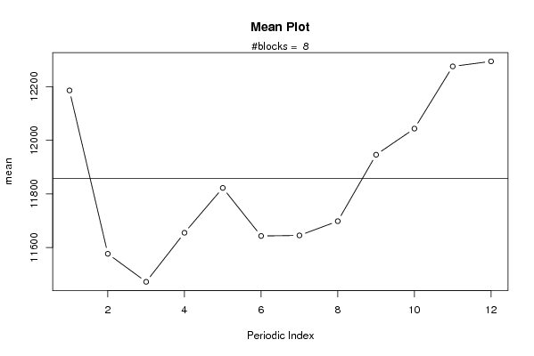
| Title produced by software | Mean Plot | ||||||||||||||||||||
| Date of computation | Mon, 28 Apr 2008 09:39:37 -0600 | ||||||||||||||||||||
| Cite this page as follows | Statistical Computations at FreeStatistics.org, Office for Research Development and Education, URL https://freestatistics.org/blog/index.php?v=date/2008/Apr/28/t1209397229xh0180yscgzvhb1.htm/, Retrieved Thu, 09 May 2024 23:14:47 +0000 | ||||||||||||||||||||
| Statistical Computations at FreeStatistics.org, Office for Research Development and Education, URL https://freestatistics.org/blog/index.php?pk=10921, Retrieved Thu, 09 May 2024 23:14:47 +0000 | |||||||||||||||||||||
| QR Codes: | |||||||||||||||||||||
|
| |||||||||||||||||||||
| Original text written by user: | Bron: belgostat | ||||||||||||||||||||
| IsPrivate? | No (this computation is public) | ||||||||||||||||||||
| User-defined keywords | Periode: januari 2000 - januari 2008 | ||||||||||||||||||||
| Estimated Impact | 227 | ||||||||||||||||||||
Tree of Dependent Computations | |||||||||||||||||||||
| Family? (F = Feedback message, R = changed R code, M = changed R Module, P = changed Parameters, D = changed Data) | |||||||||||||||||||||
| - [] [Laurane Poti� -Go...] [-0001-11-30 00:00:00] [0ca0344e1eb5e8a1a2e930e86c51900c] - RMPD [Mean Plot] [Laurane Poti� -Go...] [2008-04-28 15:39:37] [8c9b3412c86ca5b785d4e204c3e8d338] [Current] | |||||||||||||||||||||
| Feedback Forum | |||||||||||||||||||||
Post a new message | |||||||||||||||||||||
Dataset | |||||||||||||||||||||
| Dataseries X: | |||||||||||||||||||||
9026 9787 9536 9490 9736 9694 9647 9753 10070 10137 9984 9732 9103 9155 9308 9394 9948 10177 10002 9728 10002 10063 10018 9960 10236 10893 10756 10940 10997 10827 10166 10186 10457 10368 10244 10511 10812 10738 10171 9721 9897 9828 9924 10371 10846 10413 10709 10662 10570 10297 10635 10872 10296 10383 10431 10574 10653 10805 10872 10625 10407 10463 10556 10646 10702 11353 11346 11451 11964 12574 13031 13812 14544 14931 14886 16005 17064 15168 16050 15839 15137 14954 15648 15305 15579 16348 15928 16171 15937 15713 15594 15683 16438 17032 17696 17745 19394 | |||||||||||||||||||||
Tables (Output of Computation) | |||||||||||||||||||||
| |||||||||||||||||||||
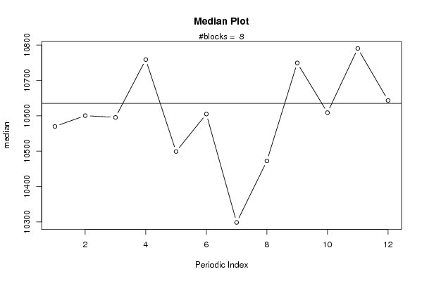
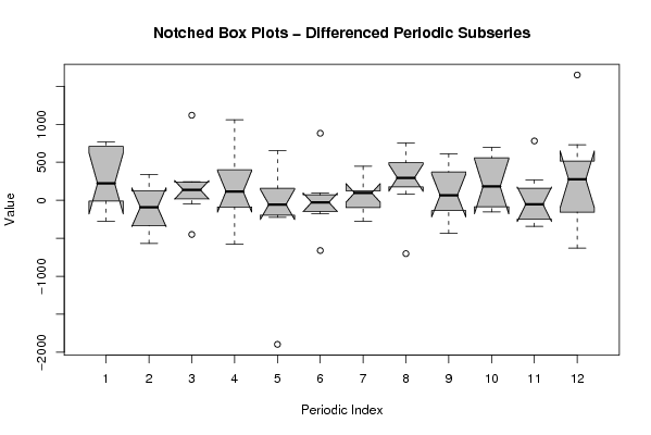
Figures (Output of Computation) | |||||||||||||||||||||
Input Parameters & R Code | |||||||||||||||||||||
| Parameters (Session): | |||||||||||||||||||||
| par1 = 12 ; | |||||||||||||||||||||
| Parameters (R input): | |||||||||||||||||||||
| par1 = 12 ; | |||||||||||||||||||||
| R code (references can be found in the software module): | |||||||||||||||||||||
par1 <- as.numeric(par1) | |||||||||||||||||||||