Free Statistics
of Irreproducible Research!
Description of Statistical Computation | |||||||||||||||||||||
|---|---|---|---|---|---|---|---|---|---|---|---|---|---|---|---|---|---|---|---|---|---|
| Author's title | |||||||||||||||||||||
| Author | *Unverified author* | ||||||||||||||||||||
| R Software Module | rwasp_meanplot.wasp | ||||||||||||||||||||
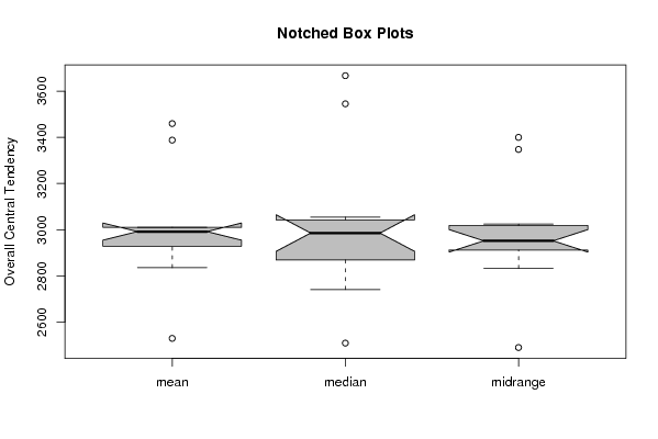
| Title produced by software | Mean Plot | ||||||||||||||||||||
| Date of computation | Mon, 28 Apr 2008 14:31:41 -0600 | ||||||||||||||||||||
| Cite this page as follows | Statistical Computations at FreeStatistics.org, Office for Research Development and Education, URL https://freestatistics.org/blog/index.php?v=date/2008/Apr/28/t1209414746c8eq6g54ta6x0dt.htm/, Retrieved Fri, 10 May 2024 13:52:24 +0000 | ||||||||||||||||||||
| Statistical Computations at FreeStatistics.org, Office for Research Development and Education, URL https://freestatistics.org/blog/index.php?pk=11005, Retrieved Fri, 10 May 2024 13:52:24 +0000 | |||||||||||||||||||||
| QR Codes: | |||||||||||||||||||||
|
| |||||||||||||||||||||
| Original text written by user: | |||||||||||||||||||||
| IsPrivate? | No (this computation is public) | ||||||||||||||||||||
| User-defined keywords | |||||||||||||||||||||
| Estimated Impact | 212 | ||||||||||||||||||||
Tree of Dependent Computations | |||||||||||||||||||||
| Family? (F = Feedback message, R = changed R code, M = changed R Module, P = changed Parameters, D = changed Data) | |||||||||||||||||||||
| - [Mean Plot] [Bouwvergunningen] [2008-04-28 20:31:41] [8e49e33bff217c9d761ee51a4d4e5949] [Current] - RM D [Standard Deviation Plot] [Bouwvergunningen] [2008-05-12 21:49:58] [70836ebc47039e6a5440e0357610e663] - RMPD [Standard Deviation-Mean Plot] [Bouwvergunningen] [2008-05-12 21:51:09] [70836ebc47039e6a5440e0357610e663] - PD [Standard Deviation-Mean Plot] [Bouwvergunningen] [2008-05-28 10:17:42] [74be16979710d4c4e7c6647856088456] | |||||||||||||||||||||
| Feedback Forum | |||||||||||||||||||||
Post a new message | |||||||||||||||||||||
Dataset | |||||||||||||||||||||
| Dataseries X: | |||||||||||||||||||||
2434 2637 1831 1851 1839 2609 2417 2394 2372 2717 2998 2538 3007 2475 2175 2465 2279 2323 2746 2601 2486 2718 2646 2551 2712 2606 2365 3533 3509 2912 3599 2719 2869 4085 2686 2545 3071 3388 2652 3190 2884 3295 3818 3226 3953 3810 2877 3515 3708 3450 3360 4098 4374 3703 4257 3487 3659 3904 2957 3320 3420 3500 2791 2919 3179 3016 3492 3034 2612 3525 2846 3212 2591 | |||||||||||||||||||||
Tables (Output of Computation) | |||||||||||||||||||||
| |||||||||||||||||||||
Figures (Output of Computation) | |||||||||||||||||||||
Input Parameters & R Code | |||||||||||||||||||||
| Parameters (Session): | |||||||||||||||||||||
| par1 = 12 ; | |||||||||||||||||||||
| Parameters (R input): | |||||||||||||||||||||
| par1 = 12 ; | |||||||||||||||||||||
| R code (references can be found in the software module): | |||||||||||||||||||||
par1 <- as.numeric(par1) | |||||||||||||||||||||