Repository of Reproducible Computations

Free Statistics

of Irreproducible Research!

Author's title

Author

*The author of this computation has been verified*

R Software Module

rwasp_autocorrelation.wasp

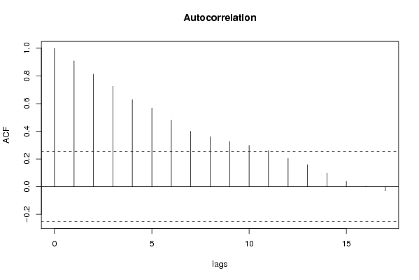
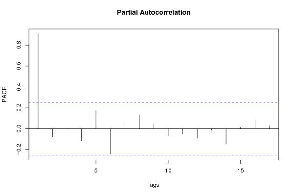
Title produced by software

(Partial) Autocorrelation Function

Date of computation

Wed, 03 Dec 2008 14:36:01 -0700

Cite this page as follows

Statistical Computations at FreeStatistics.org, Office for Research Development and Education, URL https://freestatistics.org/blog/index.php?v=date/2008/Dec/03/t1228340222tyttp97zjf4o15b.htm/, Retrieved Sun, 19 May 2024 03:09:36 +0000

Statistical Computations at FreeStatistics.org, Office for Research Development and Education, URL https://freestatistics.org/blog/index.php?pk=28894, Retrieved Sun, 19 May 2024 03:09:36 +0000

QR Codes:

Paste this QR Code to cite your computation.

Original text written by user:

IsPrivate?

No (this computation is public)

User-defined keywords

Estimated Impact

202

Family? (F = Feedback message, R = changed R code, M = changed R Module, P = changed Parameters, D = changed Data)

F     [Exercise 1.13] [Exercise 1.13 (Wo...] [2008-10-01 13:28:34] [b98453cac15ba1066b407e146608df68]
- RMPD  [Univariate Data Series] [Tijdreeks 2: Gaso...] [2008-10-20 15:56:05] [a57f5cc542637534b8bb5bcb4d37eab1]
- RMP       [(Partial) Autocorrelation Function] [Identification/es...] [2008-12-03 21:36:01] [0f30549460cf4ec26d9cf94b1fcf7789] [Current]
- RM          [Spectral Analysis] [Identification/es...] [2008-12-03 21:43:51] [a57f5cc542637534b8bb5bcb4d37eab1] 
-               [Spectral Analysis] [Identification/es...] [2008-12-03 21:47:18] [a57f5cc542637534b8bb5bcb4d37eab1] 
- RMP             [Standard Deviation-Mean Plot] [Identification/es...] [2008-12-05 10:17:50] [a57f5cc542637534b8bb5bcb4d37eab1] 
- RMP               [(Partial) Autocorrelation Function] [Identification/es...] [2008-12-05 10:30:22] [a57f5cc542637534b8bb5bcb4d37eab1] 
- RMP                 [ARIMA Backward Selection] [Identification/es...] [2008-12-05 12:40:03] [a57f5cc542637534b8bb5bcb4d37eab1] 
-   P                   [ARIMA Backward Selection] [Identification/es...] [2008-12-08 18:33:38] [a57f5cc542637534b8bb5bcb4d37eab1] 
-                         [ARIMA Backward Selection] [] [2008-12-13 20:48:17] [888addc516c3b812dd7be4bd54caa358] 

Feedback Forum

Post a new message

Dataseries X:

Download CSV

Histogram

Boxplots

0.33
0.33
0.32
0.33
0.34
0.36
0.34
0.33
0.35
0.31
0.28
0.26
0.26
0.26
0.29
0.30
0.30
0.28
0.29
0.29
0.32
0.33
0.29
0.31
0.33
0.36
0.39
0.30
0.27
0.28
0.29
0.30
0.30
0.30
0.31
0.30
0.31
0.29
0.32
0.33
0.35
0.35
0.36
0.40
0.40
0.47
0.43
0.38
0.38
0.40
0.45
0.47
0.45
0.50
0.54
0.55
0.59
0.51
0.50
0.50

Summary of computational transaction
Raw Input	view raw input (R code)
Raw Output	view raw output of R engine
Computing time	1 seconds
R Server	'George Udny Yule' @ 72.249.76.132

\begin{tabular}{lllllllll}
\hline
Summary of computational transaction \tabularnewline
Raw Input & view raw input (R code)  \tabularnewline
Raw Output & view raw output of R engine  \tabularnewline
Computing time & 1 seconds \tabularnewline
R Server & 'George Udny Yule' @ 72.249.76.132 \tabularnewline
\hline
\end{tabular}
%Source: https://freestatistics.org/blog/index.php?pk=28894&T=0

[TABLE]
[ROW][C]Summary of computational transaction[/C][/ROW]
[ROW][C]Raw Input[/C][C]view raw input (R code) [/C][/ROW]
[ROW][C]Raw Output[/C][C]view raw output of R engine [/C][/ROW]
[ROW][C]Computing time[/C][C]1 seconds[/C][/ROW]
[ROW][C]R Server[/C][C]'George Udny Yule' @ 72.249.76.132[/C][/ROW]
[/TABLE]
Source: https://freestatistics.org/blog/index.php?pk=28894&T=0

Globally Unique Identifier (entire table): ba.freestatistics.org/blog/index.php?pk=28894&T=0

As an alternative you can also use a QR Code:

The GUIDs for individual cells are displayed in the table below:

Summary of computational transaction
Raw Input	view raw input (R code)
Raw Output	view raw output of R engine
Computing time	1 seconds
R Server	'George Udny Yule' @ 72.249.76.132

Autocorrelation Function
Time lag k	ACF(k)	T-STAT	P-value
1	0.908792	7.0395	0
2	0.812682	6.295	0
3	0.725859	5.6225	0
4	0.628047	4.8648	4e-06
5	0.568982	4.4073	2.2e-05
6	0.480662	3.7232	0.000218
7	0.400186	3.0998	0.001474
8	0.36083	2.795	0.00348
9	0.325962	2.5249	0.007117
10	0.297905	2.3076	0.012245
11	0.260613	2.0187	0.023997
12	0.20387	1.5792	0.059778
13	0.158477	1.2276	0.112204
14	0.098122	0.76	0.225101
15	0.038077	0.2949	0.384529
16	0.002126	0.0165	0.493459
17	-0.030472	-0.236	0.407106

\begin{tabular}{lllllllll}
\hline
Autocorrelation Function \tabularnewline
Time lag k & ACF(k) & T-STAT & P-value \tabularnewline
1 & 0.908792 & 7.0395 & 0 \tabularnewline
2 & 0.812682 & 6.295 & 0 \tabularnewline
3 & 0.725859 & 5.6225 & 0 \tabularnewline
4 & 0.628047 & 4.8648 & 4e-06 \tabularnewline
5 & 0.568982 & 4.4073 & 2.2e-05 \tabularnewline
6 & 0.480662 & 3.7232 & 0.000218 \tabularnewline
7 & 0.400186 & 3.0998 & 0.001474 \tabularnewline
8 & 0.36083 & 2.795 & 0.00348 \tabularnewline
9 & 0.325962 & 2.5249 & 0.007117 \tabularnewline
10 & 0.297905 & 2.3076 & 0.012245 \tabularnewline
11 & 0.260613 & 2.0187 & 0.023997 \tabularnewline
12 & 0.20387 & 1.5792 & 0.059778 \tabularnewline
13 & 0.158477 & 1.2276 & 0.112204 \tabularnewline
14 & 0.098122 & 0.76 & 0.225101 \tabularnewline
15 & 0.038077 & 0.2949 & 0.384529 \tabularnewline
16 & 0.002126 & 0.0165 & 0.493459 \tabularnewline
17 & -0.030472 & -0.236 & 0.407106 \tabularnewline
\hline
\end{tabular}
%Source: https://freestatistics.org/blog/index.php?pk=28894&T=1

[TABLE]
[ROW][C]Autocorrelation Function[/C][/ROW]
[ROW][C]Time lag k[/C][C]ACF(k)[/C][C]T-STAT[/C][C]P-value[/C][/ROW]
[ROW][C]1[/C][C]0.908792[/C][C]7.0395[/C][C]0[/C][/ROW]
[ROW][C]2[/C][C]0.812682[/C][C]6.295[/C][C]0[/C][/ROW]
[ROW][C]3[/C][C]0.725859[/C][C]5.6225[/C][C]0[/C][/ROW]
[ROW][C]4[/C][C]0.628047[/C][C]4.8648[/C][C]4e-06[/C][/ROW]
[ROW][C]5[/C][C]0.568982[/C][C]4.4073[/C][C]2.2e-05[/C][/ROW]
[ROW][C]6[/C][C]0.480662[/C][C]3.7232[/C][C]0.000218[/C][/ROW]
[ROW][C]7[/C][C]0.400186[/C][C]3.0998[/C][C]0.001474[/C][/ROW]
[ROW][C]8[/C][C]0.36083[/C][C]2.795[/C][C]0.00348[/C][/ROW]
[ROW][C]9[/C][C]0.325962[/C][C]2.5249[/C][C]0.007117[/C][/ROW]
[ROW][C]10[/C][C]0.297905[/C][C]2.3076[/C][C]0.012245[/C][/ROW]
[ROW][C]11[/C][C]0.260613[/C][C]2.0187[/C][C]0.023997[/C][/ROW]
[ROW][C]12[/C][C]0.20387[/C][C]1.5792[/C][C]0.059778[/C][/ROW]
[ROW][C]13[/C][C]0.158477[/C][C]1.2276[/C][C]0.112204[/C][/ROW]
[ROW][C]14[/C][C]0.098122[/C][C]0.76[/C][C]0.225101[/C][/ROW]
[ROW][C]15[/C][C]0.038077[/C][C]0.2949[/C][C]0.384529[/C][/ROW]
[ROW][C]16[/C][C]0.002126[/C][C]0.0165[/C][C]0.493459[/C][/ROW]
[ROW][C]17[/C][C]-0.030472[/C][C]-0.236[/C][C]0.407106[/C][/ROW]
[/TABLE]
Source: https://freestatistics.org/blog/index.php?pk=28894&T=1

Globally Unique Identifier (entire table): ba.freestatistics.org/blog/index.php?pk=28894&T=1

As an alternative you can also use a QR Code:

The GUIDs for individual cells are displayed in the table below:

Autocorrelation Function
Time lag k	ACF(k)	T-STAT	P-value
1	0.908792	7.0395	0
2	0.812682	6.295	0
3	0.725859	5.6225	0
4	0.628047	4.8648	4e-06
5	0.568982	4.4073	2.2e-05
6	0.480662	3.7232	0.000218
7	0.400186	3.0998	0.001474
8	0.36083	2.795	0.00348
9	0.325962	2.5249	0.007117
10	0.297905	2.3076	0.012245
11	0.260613	2.0187	0.023997
12	0.20387	1.5792	0.059778
13	0.158477	1.2276	0.112204
14	0.098122	0.76	0.225101
15	0.038077	0.2949	0.384529
16	0.002126	0.0165	0.493459
17	-0.030472	-0.236	0.407106

Partial Autocorrelation Function
Time lag k	PACF(k)	T-STAT	P-value
1	0.908792	7.0395	0
2	-0.075937	-0.5882	0.279302
3	0.001314	0.0102	0.495956
4	-0.116758	-0.9044	0.184699
5	0.173159	1.3413	0.092442
6	-0.2423	-1.8768	0.032702
7	0.04867	0.377	0.353753
8	0.130348	1.0097	0.158353
9	0.047733	0.3697	0.356441
10	-0.068716	-0.5323	0.298251
11	-0.049941	-0.3868	0.350121
12	-0.090084	-0.6978	0.244002
13	-0.014709	-0.1139	0.454836
14	-0.147063	-1.1391	0.129585
15	0.011986	0.0928	0.46317
16	0.083131	0.6439	0.261037
17	0.028699	0.2223	0.412416

\begin{tabular}{lllllllll}
\hline
Partial Autocorrelation Function \tabularnewline
Time lag k & PACF(k) & T-STAT & P-value \tabularnewline
1 & 0.908792 & 7.0395 & 0 \tabularnewline
2 & -0.075937 & -0.5882 & 0.279302 \tabularnewline
3 & 0.001314 & 0.0102 & 0.495956 \tabularnewline
4 & -0.116758 & -0.9044 & 0.184699 \tabularnewline
5 & 0.173159 & 1.3413 & 0.092442 \tabularnewline
6 & -0.2423 & -1.8768 & 0.032702 \tabularnewline
7 & 0.04867 & 0.377 & 0.353753 \tabularnewline
8 & 0.130348 & 1.0097 & 0.158353 \tabularnewline
9 & 0.047733 & 0.3697 & 0.356441 \tabularnewline
10 & -0.068716 & -0.5323 & 0.298251 \tabularnewline
11 & -0.049941 & -0.3868 & 0.350121 \tabularnewline
12 & -0.090084 & -0.6978 & 0.244002 \tabularnewline
13 & -0.014709 & -0.1139 & 0.454836 \tabularnewline
14 & -0.147063 & -1.1391 & 0.129585 \tabularnewline
15 & 0.011986 & 0.0928 & 0.46317 \tabularnewline
16 & 0.083131 & 0.6439 & 0.261037 \tabularnewline
17 & 0.028699 & 0.2223 & 0.412416 \tabularnewline
\hline
\end{tabular}
%Source: https://freestatistics.org/blog/index.php?pk=28894&T=2

[TABLE]
[ROW][C]Partial Autocorrelation Function[/C][/ROW]
[ROW][C]Time lag k[/C][C]PACF(k)[/C][C]T-STAT[/C][C]P-value[/C][/ROW]
[ROW][C]1[/C][C]0.908792[/C][C]7.0395[/C][C]0[/C][/ROW]
[ROW][C]2[/C][C]-0.075937[/C][C]-0.5882[/C][C]0.279302[/C][/ROW]
[ROW][C]3[/C][C]0.001314[/C][C]0.0102[/C][C]0.495956[/C][/ROW]
[ROW][C]4[/C][C]-0.116758[/C][C]-0.9044[/C][C]0.184699[/C][/ROW]
[ROW][C]5[/C][C]0.173159[/C][C]1.3413[/C][C]0.092442[/C][/ROW]
[ROW][C]6[/C][C]-0.2423[/C][C]-1.8768[/C][C]0.032702[/C][/ROW]
[ROW][C]7[/C][C]0.04867[/C][C]0.377[/C][C]0.353753[/C][/ROW]
[ROW][C]8[/C][C]0.130348[/C][C]1.0097[/C][C]0.158353[/C][/ROW]
[ROW][C]9[/C][C]0.047733[/C][C]0.3697[/C][C]0.356441[/C][/ROW]
[ROW][C]10[/C][C]-0.068716[/C][C]-0.5323[/C][C]0.298251[/C][/ROW]
[ROW][C]11[/C][C]-0.049941[/C][C]-0.3868[/C][C]0.350121[/C][/ROW]
[ROW][C]12[/C][C]-0.090084[/C][C]-0.6978[/C][C]0.244002[/C][/ROW]
[ROW][C]13[/C][C]-0.014709[/C][C]-0.1139[/C][C]0.454836[/C][/ROW]
[ROW][C]14[/C][C]-0.147063[/C][C]-1.1391[/C][C]0.129585[/C][/ROW]
[ROW][C]15[/C][C]0.011986[/C][C]0.0928[/C][C]0.46317[/C][/ROW]
[ROW][C]16[/C][C]0.083131[/C][C]0.6439[/C][C]0.261037[/C][/ROW]
[ROW][C]17[/C][C]0.028699[/C][C]0.2223[/C][C]0.412416[/C][/ROW]
[/TABLE]
Source: https://freestatistics.org/blog/index.php?pk=28894&T=2

Globally Unique Identifier (entire table): ba.freestatistics.org/blog/index.php?pk=28894&T=2

As an alternative you can also use a QR Code:

The GUIDs for individual cells are displayed in the table below:

Partial Autocorrelation Function
Time lag k	PACF(k)	T-STAT	P-value
1	0.908792	7.0395	0
2	-0.075937	-0.5882	0.279302
3	0.001314	0.0102	0.495956
4	-0.116758	-0.9044	0.184699
5	0.173159	1.3413	0.092442
6	-0.2423	-1.8768	0.032702
7	0.04867	0.377	0.353753
8	0.130348	1.0097	0.158353
9	0.047733	0.3697	0.356441
10	-0.068716	-0.5323	0.298251
11	-0.049941	-0.3868	0.350121
12	-0.090084	-0.6978	0.244002
13	-0.014709	-0.1139	0.454836
14	-0.147063	-1.1391	0.129585
15	0.011986	0.0928	0.46317
16	0.083131	0.6439	0.261037
17	0.028699	0.2223	0.412416

Figure 1

PNG link

Postscript link

PDF link

Figure 2

PNG link

Postscript link

PDF link

Parameters (Session):

par1 = FALSE ; par2 = 1 ; par3 = 1 ; par4 = 1 ; par5 = 12 ; par6 = 2 ; par7 = 1 ; par8 = 2 ; par9 = 1 ;

Parameters (R input):

par1 = Default ; par2 = 1 ; par3 = 0 ; par4 = 0 ; par5 = 12 ;

R code (references can be found in the software module):

if (par1 == 'Default') {
par1 = 10*log10(length(x))
} else {
par1 <- as.numeric(par1)
}
par2 <- as.numeric(par2)
par3 <- as.numeric(par3)
par4 <- as.numeric(par4)
par5 <- as.numeric(par5)
if (par2 == 0) {
x <- log(x)
} else {
x <- (x ^ par2 - 1) / par2
}
if (par3 > 0) x <- diff(x,lag=1,difference=par3)
if (par4 > 0) x <- diff(x,lag=par5,difference=par4)
bitmap(file='pic1.png')
racf <- acf(x,par1,main='Autocorrelation',xlab='lags',ylab='ACF')
dev.off()
bitmap(file='pic2.png')
rpacf <- pacf(x,par1,main='Partial Autocorrelation',xlab='lags',ylab='PACF')
dev.off()
(myacf <- c(racf$acf))
(mypacf <- c(rpacf$acf))
lengthx <- length(x)
sqrtn <- sqrt(lengthx)
load(file='createtable')
a<-table.start()
a<-table.row.start(a)
a<-table.element(a,'Autocorrelation Function',4,TRUE)
a<-table.row.end(a)
a<-table.row.start(a)
a<-table.element(a,'Time lag k',header=TRUE)
a<-table.element(a,hyperlink('basics.htm','ACF(k)','click here for more information about the Autocorrelation Function'),header=TRUE)
a<-table.element(a,'T-STAT',header=TRUE)
a<-table.element(a,'P-value',header=TRUE)
a<-table.row.end(a)
for (i in 2:(par1+1)) {
a<-table.row.start(a)
a<-table.element(a,i-1,header=TRUE)
a<-table.element(a,round(myacf[i],6))
mytstat <- myacf[i]*sqrtn
a<-table.element(a,round(mytstat,4))
a<-table.element(a,round(1-pt(abs(mytstat),lengthx),6))
a<-table.row.end(a)
}
a<-table.end(a)
table.save(a,file='mytable.tab')
a<-table.start()
a<-table.row.start(a)
a<-table.element(a,'Partial Autocorrelation Function',4,TRUE)
a<-table.row.end(a)
a<-table.row.start(a)
a<-table.element(a,'Time lag k',header=TRUE)
a<-table.element(a,hyperlink('basics.htm','PACF(k)','click here for more information about the Partial Autocorrelation Function'),header=TRUE)
a<-table.element(a,'T-STAT',header=TRUE)
a<-table.element(a,'P-value',header=TRUE)
a<-table.row.end(a)
for (i in 1:par1) {
a<-table.row.start(a)
a<-table.element(a,i,header=TRUE)
a<-table.element(a,round(mypacf[i],6))
mytstat <- mypacf[i]*sqrtn
a<-table.element(a,round(mytstat,4))
a<-table.element(a,round(1-pt(abs(mytstat),lengthx),6))
a<-table.row.end(a)
}
a<-table.end(a)
table.save(a,file='mytable1.tab')

Free Statistics

Description of Statistical Computation

Tree of Dependent Computations

Dataset

Tables (Output of Computation)

Figures (Output of Computation)

Input Parameters & R Code