Repository of Reproducible Computations

Free Statistics

of Irreproducible Research!

Author's title

Author

*Unverified author*

R Software Module

rwasp_autocorrelation.wasp

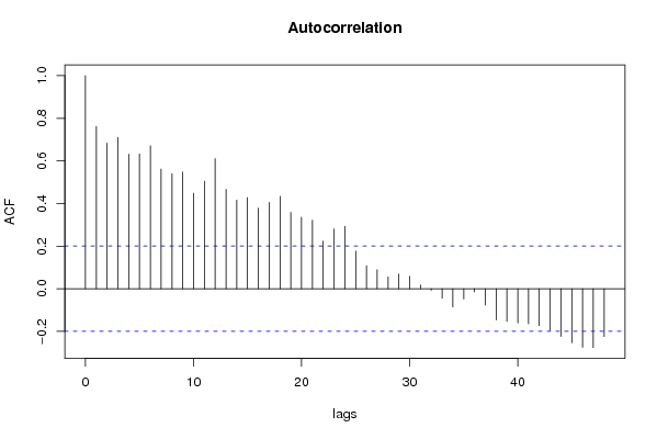
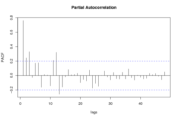
Title produced by software

(Partial) Autocorrelation Function

Date of computation

Sat, 06 Dec 2008 15:28:07 -0700

Cite this page as follows

Statistical Computations at FreeStatistics.org, Office for Research Development and Education, URL https://freestatistics.org/blog/index.php?v=date/2008/Dec/06/t1228602545xuvw87o52swahj9.htm/, Retrieved Sat, 18 May 2024 21:19:24 +0000

Statistical Computations at FreeStatistics.org, Office for Research Development and Education, URL https://freestatistics.org/blog/index.php?pk=29818, Retrieved Sat, 18 May 2024 21:19:24 +0000

QR Codes:

Paste this QR Code to cite your computation.

Original text written by user:

IsPrivate?

No (this computation is public)

User-defined keywords

Estimated Impact

170

Family? (F = Feedback message, R = changed R code, M = changed R Module, P = changed Parameters, D = changed Data)

-     [(Partial) Autocorrelation Function] ["inschrijving nie...] [2008-12-06 22:13:49] [56af8e1adaf22d814639222931271d81]
-    D    [(Partial) Autocorrelation Function] ["invoer buitenlan...] [2008-12-06 22:28:07] [cd990bb7dd50d289d8ca88511d54b252] [Current]
-   PD      [(Partial) Autocorrelation Function] [autocorr invoer m...] [2008-12-06 22:30:59] [56af8e1adaf22d814639222931271d81] 

Feedback Forum

Post a new message

Dataseries X:

Download CSV

Histogram

Boxplots

Summary of computational transaction
Raw Input	view raw input (R code)
Raw Output	view raw output of R engine
Computing time	1 seconds
R Server	'Gwilym Jenkins' @ 72.249.127.135

\begin{tabular}{lllllllll}
\hline
Summary of computational transaction \tabularnewline
Raw Input & view raw input (R code)  \tabularnewline
Raw Output & view raw output of R engine  \tabularnewline
Computing time & 1 seconds \tabularnewline
R Server & 'Gwilym Jenkins' @ 72.249.127.135 \tabularnewline
\hline
\end{tabular}
%Source: https://freestatistics.org/blog/index.php?pk=29818&T=0

[TABLE]
[ROW][C]Summary of computational transaction[/C][/ROW]
[ROW][C]Raw Input[/C][C]view raw input (R code) [/C][/ROW]
[ROW][C]Raw Output[/C][C]view raw output of R engine [/C][/ROW]
[ROW][C]Computing time[/C][C]1 seconds[/C][/ROW]
[ROW][C]R Server[/C][C]'Gwilym Jenkins' @ 72.249.127.135[/C][/ROW]
[/TABLE]
Source: https://freestatistics.org/blog/index.php?pk=29818&T=0

Globally Unique Identifier (entire table): ba.freestatistics.org/blog/index.php?pk=29818&T=0

As an alternative you can also use a QR Code:

The GUIDs for individual cells are displayed in the table below:

Summary of computational transaction
Raw Input	view raw input (R code)
Raw Output	view raw output of R engine
Computing time	1 seconds
R Server	'Gwilym Jenkins' @ 72.249.127.135

Autocorrelation Function
Time lag k	ACF(k)	T-STAT	P-value
1	0.762028	7.4663	0
2	0.683194	6.6939	0
3	0.710061	6.9571	0
4	0.630846	6.181	0
5	0.632316	6.1954	0
6	0.670622	6.5707	0
7	0.561801	5.5045	0
8	0.539507	5.2861	0
9	0.547901	5.3683	0
10	0.448016	4.3896	1.5e-05
11	0.504675	4.9448	2e-06
12	0.610703	5.9836	0
13	0.466165	4.5675	7e-06
14	0.416289	4.0788	4.7e-05
15	0.427757	4.1911	3.1e-05
16	0.378163	3.7052	0.000177
17	0.40507	3.9689	7e-05
18	0.433436	4.2468	2.5e-05
19	0.358112	3.5088	0.000344
20	0.335793	3.2901	0.000701
21	0.321748	3.1525	0.00108
22	0.223341	2.1883	0.015537
23	0.281029	2.7535	0.003526
24	0.293088	2.8717	0.002512
25	0.176728	1.7316	0.043281
26	0.10736	1.0519	0.147741
27	0.088816	0.8702	0.193177
28	0.055266	0.5415	0.29471
29	0.069086	0.6769	0.250047
30	0.058744	0.5756	0.283126
31	0.017716	0.1736	0.43128
32	-0.006754	-0.0662	0.473687
33	-0.04419	-0.433	0.333002
34	-0.08544	-0.8371	0.202299
35	-0.048093	-0.4712	0.319278
36	-0.015077	-0.1477	0.441436
37	-0.076771	-0.7522	0.226887
38	-0.14607	-1.4312	0.077812
39	-0.153414	-1.5031	0.068043
40	-0.160795	-1.5755	0.05922
41	-0.164688	-1.6136	0.054948
42	-0.173201	-1.697	0.046467
43	-0.195793	-1.9184	0.029018
44	-0.224288	-2.1976	0.015193
45	-0.253518	-2.484	0.007363
46	-0.275198	-2.6964	0.00414
47	-0.27598	-2.704	0.004052
48	-0.22477	-2.2023	0.01502

\begin{tabular}{lllllllll}
\hline
Autocorrelation Function \tabularnewline
Time lag k & ACF(k) & T-STAT & P-value \tabularnewline
1 & 0.762028 & 7.4663 & 0 \tabularnewline
2 & 0.683194 & 6.6939 & 0 \tabularnewline
3 & 0.710061 & 6.9571 & 0 \tabularnewline
4 & 0.630846 & 6.181 & 0 \tabularnewline
5 & 0.632316 & 6.1954 & 0 \tabularnewline
6 & 0.670622 & 6.5707 & 0 \tabularnewline
7 & 0.561801 & 5.5045 & 0 \tabularnewline
8 & 0.539507 & 5.2861 & 0 \tabularnewline
9 & 0.547901 & 5.3683 & 0 \tabularnewline
10 & 0.448016 & 4.3896 & 1.5e-05 \tabularnewline
11 & 0.504675 & 4.9448 & 2e-06 \tabularnewline
12 & 0.610703 & 5.9836 & 0 \tabularnewline
13 & 0.466165 & 4.5675 & 7e-06 \tabularnewline
14 & 0.416289 & 4.0788 & 4.7e-05 \tabularnewline
15 & 0.427757 & 4.1911 & 3.1e-05 \tabularnewline
16 & 0.378163 & 3.7052 & 0.000177 \tabularnewline
17 & 0.40507 & 3.9689 & 7e-05 \tabularnewline
18 & 0.433436 & 4.2468 & 2.5e-05 \tabularnewline
19 & 0.358112 & 3.5088 & 0.000344 \tabularnewline
20 & 0.335793 & 3.2901 & 0.000701 \tabularnewline
21 & 0.321748 & 3.1525 & 0.00108 \tabularnewline
22 & 0.223341 & 2.1883 & 0.015537 \tabularnewline
23 & 0.281029 & 2.7535 & 0.003526 \tabularnewline
24 & 0.293088 & 2.8717 & 0.002512 \tabularnewline
25 & 0.176728 & 1.7316 & 0.043281 \tabularnewline
26 & 0.10736 & 1.0519 & 0.147741 \tabularnewline
27 & 0.088816 & 0.8702 & 0.193177 \tabularnewline
28 & 0.055266 & 0.5415 & 0.29471 \tabularnewline
29 & 0.069086 & 0.6769 & 0.250047 \tabularnewline
30 & 0.058744 & 0.5756 & 0.283126 \tabularnewline
31 & 0.017716 & 0.1736 & 0.43128 \tabularnewline
32 & -0.006754 & -0.0662 & 0.473687 \tabularnewline
33 & -0.04419 & -0.433 & 0.333002 \tabularnewline
34 & -0.08544 & -0.8371 & 0.202299 \tabularnewline
35 & -0.048093 & -0.4712 & 0.319278 \tabularnewline
36 & -0.015077 & -0.1477 & 0.441436 \tabularnewline
37 & -0.076771 & -0.7522 & 0.226887 \tabularnewline
38 & -0.14607 & -1.4312 & 0.077812 \tabularnewline
39 & -0.153414 & -1.5031 & 0.068043 \tabularnewline
40 & -0.160795 & -1.5755 & 0.05922 \tabularnewline
41 & -0.164688 & -1.6136 & 0.054948 \tabularnewline
42 & -0.173201 & -1.697 & 0.046467 \tabularnewline
43 & -0.195793 & -1.9184 & 0.029018 \tabularnewline
44 & -0.224288 & -2.1976 & 0.015193 \tabularnewline
45 & -0.253518 & -2.484 & 0.007363 \tabularnewline
46 & -0.275198 & -2.6964 & 0.00414 \tabularnewline
47 & -0.27598 & -2.704 & 0.004052 \tabularnewline
48 & -0.22477 & -2.2023 & 0.01502 \tabularnewline
\hline
\end{tabular}
%Source: https://freestatistics.org/blog/index.php?pk=29818&T=1

[TABLE]
[ROW][C]Autocorrelation Function[/C][/ROW]
[ROW][C]Time lag k[/C][C]ACF(k)[/C][C]T-STAT[/C][C]P-value[/C][/ROW]
[ROW][C]1[/C][C]0.762028[/C][C]7.4663[/C][C]0[/C][/ROW]
[ROW][C]2[/C][C]0.683194[/C][C]6.6939[/C][C]0[/C][/ROW]
[ROW][C]3[/C][C]0.710061[/C][C]6.9571[/C][C]0[/C][/ROW]
[ROW][C]4[/C][C]0.630846[/C][C]6.181[/C][C]0[/C][/ROW]
[ROW][C]5[/C][C]0.632316[/C][C]6.1954[/C][C]0[/C][/ROW]
[ROW][C]6[/C][C]0.670622[/C][C]6.5707[/C][C]0[/C][/ROW]
[ROW][C]7[/C][C]0.561801[/C][C]5.5045[/C][C]0[/C][/ROW]
[ROW][C]8[/C][C]0.539507[/C][C]5.2861[/C][C]0[/C][/ROW]
[ROW][C]9[/C][C]0.547901[/C][C]5.3683[/C][C]0[/C][/ROW]
[ROW][C]10[/C][C]0.448016[/C][C]4.3896[/C][C]1.5e-05[/C][/ROW]
[ROW][C]11[/C][C]0.504675[/C][C]4.9448[/C][C]2e-06[/C][/ROW]
[ROW][C]12[/C][C]0.610703[/C][C]5.9836[/C][C]0[/C][/ROW]
[ROW][C]13[/C][C]0.466165[/C][C]4.5675[/C][C]7e-06[/C][/ROW]
[ROW][C]14[/C][C]0.416289[/C][C]4.0788[/C][C]4.7e-05[/C][/ROW]
[ROW][C]15[/C][C]0.427757[/C][C]4.1911[/C][C]3.1e-05[/C][/ROW]
[ROW][C]16[/C][C]0.378163[/C][C]3.7052[/C][C]0.000177[/C][/ROW]
[ROW][C]17[/C][C]0.40507[/C][C]3.9689[/C][C]7e-05[/C][/ROW]
[ROW][C]18[/C][C]0.433436[/C][C]4.2468[/C][C]2.5e-05[/C][/ROW]
[ROW][C]19[/C][C]0.358112[/C][C]3.5088[/C][C]0.000344[/C][/ROW]
[ROW][C]20[/C][C]0.335793[/C][C]3.2901[/C][C]0.000701[/C][/ROW]
[ROW][C]21[/C][C]0.321748[/C][C]3.1525[/C][C]0.00108[/C][/ROW]
[ROW][C]22[/C][C]0.223341[/C][C]2.1883[/C][C]0.015537[/C][/ROW]
[ROW][C]23[/C][C]0.281029[/C][C]2.7535[/C][C]0.003526[/C][/ROW]
[ROW][C]24[/C][C]0.293088[/C][C]2.8717[/C][C]0.002512[/C][/ROW]
[ROW][C]25[/C][C]0.176728[/C][C]1.7316[/C][C]0.043281[/C][/ROW]
[ROW][C]26[/C][C]0.10736[/C][C]1.0519[/C][C]0.147741[/C][/ROW]
[ROW][C]27[/C][C]0.088816[/C][C]0.8702[/C][C]0.193177[/C][/ROW]
[ROW][C]28[/C][C]0.055266[/C][C]0.5415[/C][C]0.29471[/C][/ROW]
[ROW][C]29[/C][C]0.069086[/C][C]0.6769[/C][C]0.250047[/C][/ROW]
[ROW][C]30[/C][C]0.058744[/C][C]0.5756[/C][C]0.283126[/C][/ROW]
[ROW][C]31[/C][C]0.017716[/C][C]0.1736[/C][C]0.43128[/C][/ROW]
[ROW][C]32[/C][C]-0.006754[/C][C]-0.0662[/C][C]0.473687[/C][/ROW]
[ROW][C]33[/C][C]-0.04419[/C][C]-0.433[/C][C]0.333002[/C][/ROW]
[ROW][C]34[/C][C]-0.08544[/C][C]-0.8371[/C][C]0.202299[/C][/ROW]
[ROW][C]35[/C][C]-0.048093[/C][C]-0.4712[/C][C]0.319278[/C][/ROW]
[ROW][C]36[/C][C]-0.015077[/C][C]-0.1477[/C][C]0.441436[/C][/ROW]
[ROW][C]37[/C][C]-0.076771[/C][C]-0.7522[/C][C]0.226887[/C][/ROW]
[ROW][C]38[/C][C]-0.14607[/C][C]-1.4312[/C][C]0.077812[/C][/ROW]
[ROW][C]39[/C][C]-0.153414[/C][C]-1.5031[/C][C]0.068043[/C][/ROW]
[ROW][C]40[/C][C]-0.160795[/C][C]-1.5755[/C][C]0.05922[/C][/ROW]
[ROW][C]41[/C][C]-0.164688[/C][C]-1.6136[/C][C]0.054948[/C][/ROW]
[ROW][C]42[/C][C]-0.173201[/C][C]-1.697[/C][C]0.046467[/C][/ROW]
[ROW][C]43[/C][C]-0.195793[/C][C]-1.9184[/C][C]0.029018[/C][/ROW]
[ROW][C]44[/C][C]-0.224288[/C][C]-2.1976[/C][C]0.015193[/C][/ROW]
[ROW][C]45[/C][C]-0.253518[/C][C]-2.484[/C][C]0.007363[/C][/ROW]
[ROW][C]46[/C][C]-0.275198[/C][C]-2.6964[/C][C]0.00414[/C][/ROW]
[ROW][C]47[/C][C]-0.27598[/C][C]-2.704[/C][C]0.004052[/C][/ROW]
[ROW][C]48[/C][C]-0.22477[/C][C]-2.2023[/C][C]0.01502[/C][/ROW]
[/TABLE]
Source: https://freestatistics.org/blog/index.php?pk=29818&T=1

Globally Unique Identifier (entire table): ba.freestatistics.org/blog/index.php?pk=29818&T=1

As an alternative you can also use a QR Code:

The GUIDs for individual cells are displayed in the table below:

Autocorrelation Function
Time lag k	ACF(k)	T-STAT	P-value
1	0.762028	7.4663	0
2	0.683194	6.6939	0
3	0.710061	6.9571	0
4	0.630846	6.181	0
5	0.632316	6.1954	0
6	0.670622	6.5707	0
7	0.561801	5.5045	0
8	0.539507	5.2861	0
9	0.547901	5.3683	0
10	0.448016	4.3896	1.5e-05
11	0.504675	4.9448	2e-06
12	0.610703	5.9836	0
13	0.466165	4.5675	7e-06
14	0.416289	4.0788	4.7e-05
15	0.427757	4.1911	3.1e-05
16	0.378163	3.7052	0.000177
17	0.40507	3.9689	7e-05
18	0.433436	4.2468	2.5e-05
19	0.358112	3.5088	0.000344
20	0.335793	3.2901	0.000701
21	0.321748	3.1525	0.00108
22	0.223341	2.1883	0.015537
23	0.281029	2.7535	0.003526
24	0.293088	2.8717	0.002512
25	0.176728	1.7316	0.043281
26	0.10736	1.0519	0.147741
27	0.088816	0.8702	0.193177
28	0.055266	0.5415	0.29471
29	0.069086	0.6769	0.250047
30	0.058744	0.5756	0.283126
31	0.017716	0.1736	0.43128
32	-0.006754	-0.0662	0.473687
33	-0.04419	-0.433	0.333002
34	-0.08544	-0.8371	0.202299
35	-0.048093	-0.4712	0.319278
36	-0.015077	-0.1477	0.441436
37	-0.076771	-0.7522	0.226887
38	-0.14607	-1.4312	0.077812
39	-0.153414	-1.5031	0.068043
40	-0.160795	-1.5755	0.05922
41	-0.164688	-1.6136	0.054948
42	-0.173201	-1.697	0.046467
43	-0.195793	-1.9184	0.029018
44	-0.224288	-2.1976	0.015193
45	-0.253518	-2.484	0.007363
46	-0.275198	-2.6964	0.00414
47	-0.27598	-2.704	0.004052
48	-0.22477	-2.2023	0.01502

Partial Autocorrelation Function
Time lag k	PACF(k)	T-STAT	P-value
1	0.762028	7.4663	0
2	0.244464	2.3953	0.009275
3	0.330827	3.2414	0.000818
4	-0.027132	-0.2658	0.395468
5	0.172652	1.6916	0.046979
6	0.177273	1.7369	0.042805
7	-0.162587	-1.593	0.057222
8	0.015641	0.1533	0.439261
9	0.008479	0.0831	0.466981
10	-0.143347	-1.4045	0.081697
11	0.211046	2.0678	0.020673
12	0.321707	3.1521	0.001082
13	-0.258221	-2.53	0.006516
14	-0.160146	-1.5691	0.059957
15	-0.018965	-0.1858	0.426489
16	0.083607	0.8192	0.207356
17	0.011956	0.1171	0.453494
18	0.016434	0.161	0.436207
19	0.031834	0.3119	0.377895
20	-0.098695	-0.967	0.167984
21	-0.056233	-0.551	0.291468
22	-0.075917	-0.7438	0.229397
23	0.076257	0.7472	0.228395
24	-0.173961	-1.7045	0.045765
25	-0.109441	-1.0723	0.143137
26	-0.149399	-1.4638	0.073257
27	0.000457	0.0045	0.498217
28	0.063385	0.621	0.268022
29	-0.020038	-0.1963	0.422385
30	-0.061388	-0.6015	0.274471
31	0.04291	0.4204	0.337554
32	-0.043687	-0.428	0.33479
33	-0.048919	-0.4793	0.316407
34	0.045221	0.4431	0.329354
35	-0.047095	-0.4614	0.322764
36	0.091878	0.9002	0.185128
37	-0.030335	-0.2972	0.383469
38	-0.063211	-0.6193	0.26858
39	0.005838	0.0572	0.477253
40	-0.024427	-0.2393	0.405677
41	-0.047797	-0.4683	0.32031
42	-0.039048	-0.3826	0.351436
43	0.03035	0.2974	0.383415
44	0.013732	0.1345	0.446626
45	0.029449	0.2885	0.386779
46	-0.01021	-0.1	0.460262
47	-0.058315	-0.5714	0.284544
48	0.051323	0.5029	0.308107

\begin{tabular}{lllllllll}
\hline
Partial Autocorrelation Function \tabularnewline
Time lag k & PACF(k) & T-STAT & P-value \tabularnewline
1 & 0.762028 & 7.4663 & 0 \tabularnewline
2 & 0.244464 & 2.3953 & 0.009275 \tabularnewline
3 & 0.330827 & 3.2414 & 0.000818 \tabularnewline
4 & -0.027132 & -0.2658 & 0.395468 \tabularnewline
5 & 0.172652 & 1.6916 & 0.046979 \tabularnewline
6 & 0.177273 & 1.7369 & 0.042805 \tabularnewline
7 & -0.162587 & -1.593 & 0.057222 \tabularnewline
8 & 0.015641 & 0.1533 & 0.439261 \tabularnewline
9 & 0.008479 & 0.0831 & 0.466981 \tabularnewline
10 & -0.143347 & -1.4045 & 0.081697 \tabularnewline
11 & 0.211046 & 2.0678 & 0.020673 \tabularnewline
12 & 0.321707 & 3.1521 & 0.001082 \tabularnewline
13 & -0.258221 & -2.53 & 0.006516 \tabularnewline
14 & -0.160146 & -1.5691 & 0.059957 \tabularnewline
15 & -0.018965 & -0.1858 & 0.426489 \tabularnewline
16 & 0.083607 & 0.8192 & 0.207356 \tabularnewline
17 & 0.011956 & 0.1171 & 0.453494 \tabularnewline
18 & 0.016434 & 0.161 & 0.436207 \tabularnewline
19 & 0.031834 & 0.3119 & 0.377895 \tabularnewline
20 & -0.098695 & -0.967 & 0.167984 \tabularnewline
21 & -0.056233 & -0.551 & 0.291468 \tabularnewline
22 & -0.075917 & -0.7438 & 0.229397 \tabularnewline
23 & 0.076257 & 0.7472 & 0.228395 \tabularnewline
24 & -0.173961 & -1.7045 & 0.045765 \tabularnewline
25 & -0.109441 & -1.0723 & 0.143137 \tabularnewline
26 & -0.149399 & -1.4638 & 0.073257 \tabularnewline
27 & 0.000457 & 0.0045 & 0.498217 \tabularnewline
28 & 0.063385 & 0.621 & 0.268022 \tabularnewline
29 & -0.020038 & -0.1963 & 0.422385 \tabularnewline
30 & -0.061388 & -0.6015 & 0.274471 \tabularnewline
31 & 0.04291 & 0.4204 & 0.337554 \tabularnewline
32 & -0.043687 & -0.428 & 0.33479 \tabularnewline
33 & -0.048919 & -0.4793 & 0.316407 \tabularnewline
34 & 0.045221 & 0.4431 & 0.329354 \tabularnewline
35 & -0.047095 & -0.4614 & 0.322764 \tabularnewline
36 & 0.091878 & 0.9002 & 0.185128 \tabularnewline
37 & -0.030335 & -0.2972 & 0.383469 \tabularnewline
38 & -0.063211 & -0.6193 & 0.26858 \tabularnewline
39 & 0.005838 & 0.0572 & 0.477253 \tabularnewline
40 & -0.024427 & -0.2393 & 0.405677 \tabularnewline
41 & -0.047797 & -0.4683 & 0.32031 \tabularnewline
42 & -0.039048 & -0.3826 & 0.351436 \tabularnewline
43 & 0.03035 & 0.2974 & 0.383415 \tabularnewline
44 & 0.013732 & 0.1345 & 0.446626 \tabularnewline
45 & 0.029449 & 0.2885 & 0.386779 \tabularnewline
46 & -0.01021 & -0.1 & 0.460262 \tabularnewline
47 & -0.058315 & -0.5714 & 0.284544 \tabularnewline
48 & 0.051323 & 0.5029 & 0.308107 \tabularnewline
\hline
\end{tabular}
%Source: https://freestatistics.org/blog/index.php?pk=29818&T=2

[TABLE]
[ROW][C]Partial Autocorrelation Function[/C][/ROW]
[ROW][C]Time lag k[/C][C]PACF(k)[/C][C]T-STAT[/C][C]P-value[/C][/ROW]
[ROW][C]1[/C][C]0.762028[/C][C]7.4663[/C][C]0[/C][/ROW]
[ROW][C]2[/C][C]0.244464[/C][C]2.3953[/C][C]0.009275[/C][/ROW]
[ROW][C]3[/C][C]0.330827[/C][C]3.2414[/C][C]0.000818[/C][/ROW]
[ROW][C]4[/C][C]-0.027132[/C][C]-0.2658[/C][C]0.395468[/C][/ROW]
[ROW][C]5[/C][C]0.172652[/C][C]1.6916[/C][C]0.046979[/C][/ROW]
[ROW][C]6[/C][C]0.177273[/C][C]1.7369[/C][C]0.042805[/C][/ROW]
[ROW][C]7[/C][C]-0.162587[/C][C]-1.593[/C][C]0.057222[/C][/ROW]
[ROW][C]8[/C][C]0.015641[/C][C]0.1533[/C][C]0.439261[/C][/ROW]
[ROW][C]9[/C][C]0.008479[/C][C]0.0831[/C][C]0.466981[/C][/ROW]
[ROW][C]10[/C][C]-0.143347[/C][C]-1.4045[/C][C]0.081697[/C][/ROW]
[ROW][C]11[/C][C]0.211046[/C][C]2.0678[/C][C]0.020673[/C][/ROW]
[ROW][C]12[/C][C]0.321707[/C][C]3.1521[/C][C]0.001082[/C][/ROW]
[ROW][C]13[/C][C]-0.258221[/C][C]-2.53[/C][C]0.006516[/C][/ROW]
[ROW][C]14[/C][C]-0.160146[/C][C]-1.5691[/C][C]0.059957[/C][/ROW]
[ROW][C]15[/C][C]-0.018965[/C][C]-0.1858[/C][C]0.426489[/C][/ROW]
[ROW][C]16[/C][C]0.083607[/C][C]0.8192[/C][C]0.207356[/C][/ROW]
[ROW][C]17[/C][C]0.011956[/C][C]0.1171[/C][C]0.453494[/C][/ROW]
[ROW][C]18[/C][C]0.016434[/C][C]0.161[/C][C]0.436207[/C][/ROW]
[ROW][C]19[/C][C]0.031834[/C][C]0.3119[/C][C]0.377895[/C][/ROW]
[ROW][C]20[/C][C]-0.098695[/C][C]-0.967[/C][C]0.167984[/C][/ROW]
[ROW][C]21[/C][C]-0.056233[/C][C]-0.551[/C][C]0.291468[/C][/ROW]
[ROW][C]22[/C][C]-0.075917[/C][C]-0.7438[/C][C]0.229397[/C][/ROW]
[ROW][C]23[/C][C]0.076257[/C][C]0.7472[/C][C]0.228395[/C][/ROW]
[ROW][C]24[/C][C]-0.173961[/C][C]-1.7045[/C][C]0.045765[/C][/ROW]
[ROW][C]25[/C][C]-0.109441[/C][C]-1.0723[/C][C]0.143137[/C][/ROW]
[ROW][C]26[/C][C]-0.149399[/C][C]-1.4638[/C][C]0.073257[/C][/ROW]
[ROW][C]27[/C][C]0.000457[/C][C]0.0045[/C][C]0.498217[/C][/ROW]
[ROW][C]28[/C][C]0.063385[/C][C]0.621[/C][C]0.268022[/C][/ROW]
[ROW][C]29[/C][C]-0.020038[/C][C]-0.1963[/C][C]0.422385[/C][/ROW]
[ROW][C]30[/C][C]-0.061388[/C][C]-0.6015[/C][C]0.274471[/C][/ROW]
[ROW][C]31[/C][C]0.04291[/C][C]0.4204[/C][C]0.337554[/C][/ROW]
[ROW][C]32[/C][C]-0.043687[/C][C]-0.428[/C][C]0.33479[/C][/ROW]
[ROW][C]33[/C][C]-0.048919[/C][C]-0.4793[/C][C]0.316407[/C][/ROW]
[ROW][C]34[/C][C]0.045221[/C][C]0.4431[/C][C]0.329354[/C][/ROW]
[ROW][C]35[/C][C]-0.047095[/C][C]-0.4614[/C][C]0.322764[/C][/ROW]
[ROW][C]36[/C][C]0.091878[/C][C]0.9002[/C][C]0.185128[/C][/ROW]
[ROW][C]37[/C][C]-0.030335[/C][C]-0.2972[/C][C]0.383469[/C][/ROW]
[ROW][C]38[/C][C]-0.063211[/C][C]-0.6193[/C][C]0.26858[/C][/ROW]
[ROW][C]39[/C][C]0.005838[/C][C]0.0572[/C][C]0.477253[/C][/ROW]
[ROW][C]40[/C][C]-0.024427[/C][C]-0.2393[/C][C]0.405677[/C][/ROW]
[ROW][C]41[/C][C]-0.047797[/C][C]-0.4683[/C][C]0.32031[/C][/ROW]
[ROW][C]42[/C][C]-0.039048[/C][C]-0.3826[/C][C]0.351436[/C][/ROW]
[ROW][C]43[/C][C]0.03035[/C][C]0.2974[/C][C]0.383415[/C][/ROW]
[ROW][C]44[/C][C]0.013732[/C][C]0.1345[/C][C]0.446626[/C][/ROW]
[ROW][C]45[/C][C]0.029449[/C][C]0.2885[/C][C]0.386779[/C][/ROW]
[ROW][C]46[/C][C]-0.01021[/C][C]-0.1[/C][C]0.460262[/C][/ROW]
[ROW][C]47[/C][C]-0.058315[/C][C]-0.5714[/C][C]0.284544[/C][/ROW]
[ROW][C]48[/C][C]0.051323[/C][C]0.5029[/C][C]0.308107[/C][/ROW]
[/TABLE]
Source: https://freestatistics.org/blog/index.php?pk=29818&T=2

Globally Unique Identifier (entire table): ba.freestatistics.org/blog/index.php?pk=29818&T=2

As an alternative you can also use a QR Code:

The GUIDs for individual cells are displayed in the table below:

Partial Autocorrelation Function
Time lag k	PACF(k)	T-STAT	P-value
1	0.762028	7.4663	0
2	0.244464	2.3953	0.009275
3	0.330827	3.2414	0.000818
4	-0.027132	-0.2658	0.395468
5	0.172652	1.6916	0.046979
6	0.177273	1.7369	0.042805
7	-0.162587	-1.593	0.057222
8	0.015641	0.1533	0.439261
9	0.008479	0.0831	0.466981
10	-0.143347	-1.4045	0.081697
11	0.211046	2.0678	0.020673
12	0.321707	3.1521	0.001082
13	-0.258221	-2.53	0.006516
14	-0.160146	-1.5691	0.059957
15	-0.018965	-0.1858	0.426489
16	0.083607	0.8192	0.207356
17	0.011956	0.1171	0.453494
18	0.016434	0.161	0.436207
19	0.031834	0.3119	0.377895
20	-0.098695	-0.967	0.167984
21	-0.056233	-0.551	0.291468
22	-0.075917	-0.7438	0.229397
23	0.076257	0.7472	0.228395
24	-0.173961	-1.7045	0.045765
25	-0.109441	-1.0723	0.143137
26	-0.149399	-1.4638	0.073257
27	0.000457	0.0045	0.498217
28	0.063385	0.621	0.268022
29	-0.020038	-0.1963	0.422385
30	-0.061388	-0.6015	0.274471
31	0.04291	0.4204	0.337554
32	-0.043687	-0.428	0.33479
33	-0.048919	-0.4793	0.316407
34	0.045221	0.4431	0.329354
35	-0.047095	-0.4614	0.322764
36	0.091878	0.9002	0.185128
37	-0.030335	-0.2972	0.383469
38	-0.063211	-0.6193	0.26858
39	0.005838	0.0572	0.477253
40	-0.024427	-0.2393	0.405677
41	-0.047797	-0.4683	0.32031
42	-0.039048	-0.3826	0.351436
43	0.03035	0.2974	0.383415
44	0.013732	0.1345	0.446626
45	0.029449	0.2885	0.386779
46	-0.01021	-0.1	0.460262
47	-0.058315	-0.5714	0.284544
48	0.051323	0.5029	0.308107

Figure 1

PNG link

Postscript link

PDF link

Figure 2

PNG link

Postscript link

PDF link

Parameters (Session):

par1 = 48 ; par2 = 1 ; par3 = 0 ; par4 = 0 ; par5 = 12 ;

Parameters (R input):

par1 = 48 ; par2 = 1 ; par3 = 0 ; par4 = 0 ; par5 = 12 ;

R code (references can be found in the software module):

if (par1 == 'Default') {
par1 = 10*log10(length(x))
} else {
par1 <- as.numeric(par1)
}
par2 <- as.numeric(par2)
par3 <- as.numeric(par3)
par4 <- as.numeric(par4)
par5 <- as.numeric(par5)
if (par2 == 0) {
x <- log(x)
} else {
x <- (x ^ par2 - 1) / par2
}
if (par3 > 0) x <- diff(x,lag=1,difference=par3)
if (par4 > 0) x <- diff(x,lag=par5,difference=par4)
bitmap(file='pic1.png')
racf <- acf(x,par1,main='Autocorrelation',xlab='lags',ylab='ACF')
dev.off()
bitmap(file='pic2.png')
rpacf <- pacf(x,par1,main='Partial Autocorrelation',xlab='lags',ylab='PACF')
dev.off()
(myacf <- c(racf$acf))
(mypacf <- c(rpacf$acf))
lengthx <- length(x)
sqrtn <- sqrt(lengthx)
load(file='createtable')
a<-table.start()
a<-table.row.start(a)
a<-table.element(a,'Autocorrelation Function',4,TRUE)
a<-table.row.end(a)
a<-table.row.start(a)
a<-table.element(a,'Time lag k',header=TRUE)
a<-table.element(a,hyperlink('basics.htm','ACF(k)','click here for more information about the Autocorrelation Function'),header=TRUE)
a<-table.element(a,'T-STAT',header=TRUE)
a<-table.element(a,'P-value',header=TRUE)
a<-table.row.end(a)
for (i in 2:(par1+1)) {
a<-table.row.start(a)
a<-table.element(a,i-1,header=TRUE)
a<-table.element(a,round(myacf[i],6))
mytstat <- myacf[i]*sqrtn
a<-table.element(a,round(mytstat,4))
a<-table.element(a,round(1-pt(abs(mytstat),lengthx),6))
a<-table.row.end(a)
}
a<-table.end(a)
table.save(a,file='mytable.tab')
a<-table.start()
a<-table.row.start(a)
a<-table.element(a,'Partial Autocorrelation Function',4,TRUE)
a<-table.row.end(a)
a<-table.row.start(a)
a<-table.element(a,'Time lag k',header=TRUE)
a<-table.element(a,hyperlink('basics.htm','PACF(k)','click here for more information about the Partial Autocorrelation Function'),header=TRUE)
a<-table.element(a,'T-STAT',header=TRUE)
a<-table.element(a,'P-value',header=TRUE)
a<-table.row.end(a)
for (i in 1:par1) {
a<-table.row.start(a)
a<-table.element(a,i,header=TRUE)
a<-table.element(a,round(mypacf[i],6))
mytstat <- mypacf[i]*sqrtn
a<-table.element(a,round(mytstat,4))
a<-table.element(a,round(1-pt(abs(mytstat),lengthx),6))
a<-table.row.end(a)
}
a<-table.end(a)
table.save(a,file='mytable1.tab')

Free Statistics

Description of Statistical Computation

Tree of Dependent Computations

Dataset

Tables (Output of Computation)

Figures (Output of Computation)

Input Parameters & R Code