Free Statistics
of Irreproducible Research!
Description of Statistical Computation | |||||||||||||||||||||
|---|---|---|---|---|---|---|---|---|---|---|---|---|---|---|---|---|---|---|---|---|---|
| Author's title | |||||||||||||||||||||
| Author | *Unverified author* | ||||||||||||||||||||
| R Software Module | rwasp_sdplot.wasp | ||||||||||||||||||||
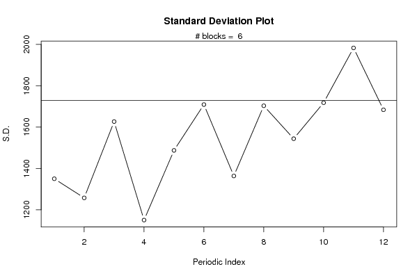
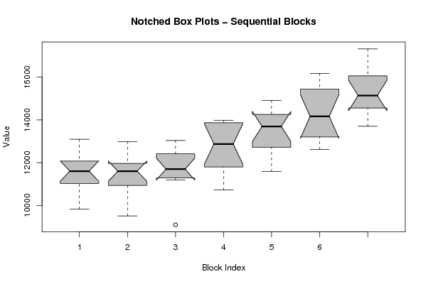
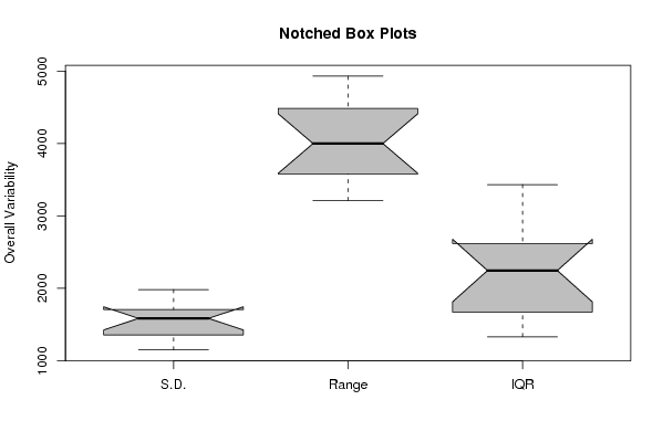
| Title produced by software | Standard Deviation Plot | ||||||||||||||||||||
| Date of computation | Mon, 12 May 2008 13:51:47 -0600 | ||||||||||||||||||||
| Cite this page as follows | Statistical Computations at FreeStatistics.org, Office for Research Development and Education, URL https://freestatistics.org/blog/index.php?v=date/2008/May/12/t1210621948zn1j4g99qgxyc2o.htm/, Retrieved Tue, 14 May 2024 16:22:16 +0000 | ||||||||||||||||||||
| Statistical Computations at FreeStatistics.org, Office for Research Development and Education, URL https://freestatistics.org/blog/index.php?pk=12428, Retrieved Tue, 14 May 2024 16:22:16 +0000 | |||||||||||||||||||||
| QR Codes: | |||||||||||||||||||||
|
| |||||||||||||||||||||
| Original text written by user: | |||||||||||||||||||||
| IsPrivate? | No (this computation is public) | ||||||||||||||||||||
| User-defined keywords | |||||||||||||||||||||
| Estimated Impact | 168 | ||||||||||||||||||||
Tree of Dependent Computations | |||||||||||||||||||||
| Family? (F = Feedback message, R = changed R code, M = changed R Module, P = changed Parameters, D = changed Data) | |||||||||||||||||||||
| - [Standard Deviation Plot] [Van Passen Glenn ...] [2008-05-12 19:51:47] [7568f24034461b5d7b2d183bbb217711] [Current] - RM D [Standard Deviation-Mean Plot] [Glenn Van Passen ...] [2008-05-14 06:23:07] [447a393a477391846fb1ef840a8b4411] | |||||||||||||||||||||
| Feedback Forum | |||||||||||||||||||||
Post a new message | |||||||||||||||||||||
Dataset | |||||||||||||||||||||
| Dataseries X: | |||||||||||||||||||||
11835.70 11542.20 13093.70 11180.20 12035.70 12112.00 10875.20 9897.30 11672.10 12385.70 11405.60 9830.90 11025.10 10853.80 12252.60 11839.40 11669.10 11601.40 11178.40 9516.40 12102.80 12989.00 11610.20 10205.50 11356.20 11307.10 12648.60 11947.20 11714.10 12192.50 11268.80 9097.40 12639.80 13040.10 11687.30 11191.70 11391.90 11793.10 13933.20 12778.10 11810.30 13698.40 11956.60 10723.80 13938.90 13979.80 13807.40 12973.90 12509.80 12934.10 14908.30 13772.10 13012.60 14049.90 11816.50 11593.20 14466.20 13615.90 14733.90 13880.70 13527.50 13584.00 16170.20 13260.60 14741.90 15486.50 13154.50 12621.20 15031.60 15452.40 15428.00 13105.90 14716.80 14180.00 16202.20 14392.40 15140.60 15960.10 14729.90 13705.20 15728.50 17315.60 16152.80 | |||||||||||||||||||||
Tables (Output of Computation) | |||||||||||||||||||||
| |||||||||||||||||||||
Figures (Output of Computation) | |||||||||||||||||||||
Input Parameters & R Code | |||||||||||||||||||||
| Parameters (Session): | |||||||||||||||||||||
| par1 = 12 ; | |||||||||||||||||||||
| Parameters (R input): | |||||||||||||||||||||
| par1 = 12 ; | |||||||||||||||||||||
| R code (references can be found in the software module): | |||||||||||||||||||||
par1 <- as.numeric(par1) | |||||||||||||||||||||