Free Statistics

of Irreproducible Research!

Author's title

Author*Unverified author*
R Software Modulerwasp_exponentialsmoothing.wasp
Title produced by softwareExponential Smoothing
Date of computationSun, 25 May 2008 09:13:51 -0600
Cite this page as followsStatistical Computations at FreeStatistics.org, Office for Research Development and Education, URL https://freestatistics.org/blog/index.php?v=date/2008/May/25/t1211728471ve2cbshqkl32tb3.htm/, Retrieved Wed, 15 May 2024 09:33:13 +0000
Statistical Computations at FreeStatistics.org, Office for Research Development and Education, URL https://freestatistics.org/blog/index.php?pk=13167, Retrieved Wed, 15 May 2024 09:33:13 +0000
QR Codes:

Original text written by user:
IsPrivate?No (this computation is public)
User-defined keywords
Estimated Impact174
Family? (F = Feedback message, R = changed R code, M = changed R Module, P = changed Parameters, D = changed Data)
-       [Exponential Smoothing] [] [2008-05-25 15:13:51] [15ccabfe3b960eee2f000db554701399] [Current]
Feedback Forum

Post a new message
Dataseries X:
138463
138529
138421
138674
138848
139174
139565
139585
139500
139756
140245
140138
140224
140354
140563
141244
141597
141708
142055
142457
142429
142613
142564
142778
143086
143362
143619
143791
144088
144369
144295
144671
144846
145395
145583
145949
145915
145888
146145
145713
145913
146087
146045
145753
146260
146016
146647
146211
146248


Summary of computational transaction
Raw Inputview raw input (R code)
Raw Outputview raw output of R engine
Computing time13 seconds
R Server'Sir Ronald Aylmer Fisher' @ 193.190.124.24

\begin{tabular}{lllllllll}
\hline
Summary of computational transaction \tabularnewline
Raw Input & view raw input (R code)  \tabularnewline
Raw Output & view raw output of R engine  \tabularnewline
Computing time & 13 seconds \tabularnewline
R Server & 'Sir Ronald Aylmer Fisher' @ 193.190.124.24 \tabularnewline
\hline
\end{tabular}
%Source: https://freestatistics.org/blog/index.php?pk=13167&T=0

[TABLE]
[ROW][C]Summary of computational transaction[/C][/ROW]
[ROW][C]Raw Input[/C][C]view raw input (R code) [/C][/ROW]
[ROW][C]Raw Output[/C][C]view raw output of R engine [/C][/ROW]
[ROW][C]Computing time[/C][C]13 seconds[/C][/ROW]
[ROW][C]R Server[/C][C]'Sir Ronald Aylmer Fisher' @ 193.190.124.24[/C][/ROW]
[/TABLE]
Source: https://freestatistics.org/blog/index.php?pk=13167&T=0

Globally Unique Identifier (entire table): ba.freestatistics.org/blog/index.php?pk=13167&T=0

As an alternative you can also use a QR Code:  

The GUIDs for individual cells are displayed in the table below:

Summary of computational transaction
Raw Inputview raw input (R code)
Raw Outputview raw output of R engine
Computing time13 seconds
R Server'Sir Ronald Aylmer Fisher' @ 193.190.124.24


Estimated Parameters of Exponential Smoothing
ParameterValue
alpha0.874555242454075
beta0.000783601938547028
gamma0.487975455959473

\begin{tabular}{lllllllll}
\hline
Estimated Parameters of Exponential Smoothing \tabularnewline
Parameter & Value \tabularnewline
alpha & 0.874555242454075 \tabularnewline
beta & 0.000783601938547028 \tabularnewline
gamma & 0.487975455959473 \tabularnewline
\hline
\end{tabular}
%Source: https://freestatistics.org/blog/index.php?pk=13167&T=1

[TABLE]
[ROW][C]Estimated Parameters of Exponential Smoothing[/C][/ROW]
[ROW][C]Parameter[/C][C]Value[/C][/ROW]
[ROW][C]alpha[/C][C]0.874555242454075[/C][/ROW]
[ROW][C]beta[/C][C]0.000783601938547028[/C][/ROW]
[ROW][C]gamma[/C][C]0.487975455959473[/C][/ROW]
[/TABLE]
Source: https://freestatistics.org/blog/index.php?pk=13167&T=1

Globally Unique Identifier (entire table): ba.freestatistics.org/blog/index.php?pk=13167&T=1

As an alternative you can also use a QR Code:  

The GUIDs for individual cells are displayed in the table below:

Estimated Parameters of Exponential Smoothing
ParameterValue
alpha0.874555242454075
beta0.000783601938547028
gamma0.487975455959473


Interpolation Forecasts of Exponential Smoothing
tObservedFittedResiduals
13140224138975.0959722221248.90402777772
14140354140195.105096103158.894903897337
15140563140522.65825088740.3417491125583
16141244141219.18276897524.8172310251393
17141597141599.563912376-2.56391237641219
18141708141723.038642881-15.0386428810889
19142055142048.9682263956.0317736050929
20142457142432.99585336824.0041466323310
21142429142394.67443017634.3255698244611
22142613142596.61151850116.388481498725
23142564142573.414529943-9.41452994258725
24142778142785.894930649-7.89493064946146
25143086143035.85759244550.1424075545219
26143362143140.978999477221.021000523207
27143619143515.869645057103.130354943016
28143791144266.660875199-475.660875199421
29144088144207.632104469-119.632104468561
30144369144227.842324653141.157675346563
31144295144691.652781137-396.65278113712
32144671144724.323479192-53.323479192477
33144846144618.66639711227.333602890023
34145395144988.093747798406.906252202083
35145583145304.906316835278.093683164945
36145949145769.178282089179.821717910847
37145915146187.247590087-272.247590086772
38145888146021.045727149-133.045727148856
39146145146078.99069997766.0093000231136
40145713146761.783766649-1048.78376664859
41145913146222.824890125-309.824890125252
42146087146092.038240267-5.03824026716757
43146045146394.343846403-349.343846403266
44145753146488.710852746-735.710852746211
45146260145802.286289967457.713710033131
46146016146383.181846860-367.181846860447
47146647146013.591720177633.408279823023
48146211146781.299047702-570.299047701585
49146248146513.868029190-265.868029189616

\begin{tabular}{lllllllll}
\hline
Interpolation Forecasts of Exponential Smoothing \tabularnewline
t & Observed & Fitted & Residuals \tabularnewline
13 & 140224 & 138975.095972222 & 1248.90402777772 \tabularnewline
14 & 140354 & 140195.105096103 & 158.894903897337 \tabularnewline
15 & 140563 & 140522.658250887 & 40.3417491125583 \tabularnewline
16 & 141244 & 141219.182768975 & 24.8172310251393 \tabularnewline
17 & 141597 & 141599.563912376 & -2.56391237641219 \tabularnewline
18 & 141708 & 141723.038642881 & -15.0386428810889 \tabularnewline
19 & 142055 & 142048.968226395 & 6.0317736050929 \tabularnewline
20 & 142457 & 142432.995853368 & 24.0041466323310 \tabularnewline
21 & 142429 & 142394.674430176 & 34.3255698244611 \tabularnewline
22 & 142613 & 142596.611518501 & 16.388481498725 \tabularnewline
23 & 142564 & 142573.414529943 & -9.41452994258725 \tabularnewline
24 & 142778 & 142785.894930649 & -7.89493064946146 \tabularnewline
25 & 143086 & 143035.857592445 & 50.1424075545219 \tabularnewline
26 & 143362 & 143140.978999477 & 221.021000523207 \tabularnewline
27 & 143619 & 143515.869645057 & 103.130354943016 \tabularnewline
28 & 143791 & 144266.660875199 & -475.660875199421 \tabularnewline
29 & 144088 & 144207.632104469 & -119.632104468561 \tabularnewline
30 & 144369 & 144227.842324653 & 141.157675346563 \tabularnewline
31 & 144295 & 144691.652781137 & -396.65278113712 \tabularnewline
32 & 144671 & 144724.323479192 & -53.323479192477 \tabularnewline
33 & 144846 & 144618.66639711 & 227.333602890023 \tabularnewline
34 & 145395 & 144988.093747798 & 406.906252202083 \tabularnewline
35 & 145583 & 145304.906316835 & 278.093683164945 \tabularnewline
36 & 145949 & 145769.178282089 & 179.821717910847 \tabularnewline
37 & 145915 & 146187.247590087 & -272.247590086772 \tabularnewline
38 & 145888 & 146021.045727149 & -133.045727148856 \tabularnewline
39 & 146145 & 146078.990699977 & 66.0093000231136 \tabularnewline
40 & 145713 & 146761.783766649 & -1048.78376664859 \tabularnewline
41 & 145913 & 146222.824890125 & -309.824890125252 \tabularnewline
42 & 146087 & 146092.038240267 & -5.03824026716757 \tabularnewline
43 & 146045 & 146394.343846403 & -349.343846403266 \tabularnewline
44 & 145753 & 146488.710852746 & -735.710852746211 \tabularnewline
45 & 146260 & 145802.286289967 & 457.713710033131 \tabularnewline
46 & 146016 & 146383.181846860 & -367.181846860447 \tabularnewline
47 & 146647 & 146013.591720177 & 633.408279823023 \tabularnewline
48 & 146211 & 146781.299047702 & -570.299047701585 \tabularnewline
49 & 146248 & 146513.868029190 & -265.868029189616 \tabularnewline
\hline
\end{tabular}
%Source: https://freestatistics.org/blog/index.php?pk=13167&T=2

[TABLE]
[ROW][C]Interpolation Forecasts of Exponential Smoothing[/C][/ROW]
[ROW][C]t[/C][C]Observed[/C][C]Fitted[/C][C]Residuals[/C][/ROW]
[ROW][C]13[/C][C]140224[/C][C]138975.095972222[/C][C]1248.90402777772[/C][/ROW]
[ROW][C]14[/C][C]140354[/C][C]140195.105096103[/C][C]158.894903897337[/C][/ROW]
[ROW][C]15[/C][C]140563[/C][C]140522.658250887[/C][C]40.3417491125583[/C][/ROW]
[ROW][C]16[/C][C]141244[/C][C]141219.182768975[/C][C]24.8172310251393[/C][/ROW]
[ROW][C]17[/C][C]141597[/C][C]141599.563912376[/C][C]-2.56391237641219[/C][/ROW]
[ROW][C]18[/C][C]141708[/C][C]141723.038642881[/C][C]-15.0386428810889[/C][/ROW]
[ROW][C]19[/C][C]142055[/C][C]142048.968226395[/C][C]6.0317736050929[/C][/ROW]
[ROW][C]20[/C][C]142457[/C][C]142432.995853368[/C][C]24.0041466323310[/C][/ROW]
[ROW][C]21[/C][C]142429[/C][C]142394.674430176[/C][C]34.3255698244611[/C][/ROW]
[ROW][C]22[/C][C]142613[/C][C]142596.611518501[/C][C]16.388481498725[/C][/ROW]
[ROW][C]23[/C][C]142564[/C][C]142573.414529943[/C][C]-9.41452994258725[/C][/ROW]
[ROW][C]24[/C][C]142778[/C][C]142785.894930649[/C][C]-7.89493064946146[/C][/ROW]
[ROW][C]25[/C][C]143086[/C][C]143035.857592445[/C][C]50.1424075545219[/C][/ROW]
[ROW][C]26[/C][C]143362[/C][C]143140.978999477[/C][C]221.021000523207[/C][/ROW]
[ROW][C]27[/C][C]143619[/C][C]143515.869645057[/C][C]103.130354943016[/C][/ROW]
[ROW][C]28[/C][C]143791[/C][C]144266.660875199[/C][C]-475.660875199421[/C][/ROW]
[ROW][C]29[/C][C]144088[/C][C]144207.632104469[/C][C]-119.632104468561[/C][/ROW]
[ROW][C]30[/C][C]144369[/C][C]144227.842324653[/C][C]141.157675346563[/C][/ROW]
[ROW][C]31[/C][C]144295[/C][C]144691.652781137[/C][C]-396.65278113712[/C][/ROW]
[ROW][C]32[/C][C]144671[/C][C]144724.323479192[/C][C]-53.323479192477[/C][/ROW]
[ROW][C]33[/C][C]144846[/C][C]144618.66639711[/C][C]227.333602890023[/C][/ROW]
[ROW][C]34[/C][C]145395[/C][C]144988.093747798[/C][C]406.906252202083[/C][/ROW]
[ROW][C]35[/C][C]145583[/C][C]145304.906316835[/C][C]278.093683164945[/C][/ROW]
[ROW][C]36[/C][C]145949[/C][C]145769.178282089[/C][C]179.821717910847[/C][/ROW]
[ROW][C]37[/C][C]145915[/C][C]146187.247590087[/C][C]-272.247590086772[/C][/ROW]
[ROW][C]38[/C][C]145888[/C][C]146021.045727149[/C][C]-133.045727148856[/C][/ROW]
[ROW][C]39[/C][C]146145[/C][C]146078.990699977[/C][C]66.0093000231136[/C][/ROW]
[ROW][C]40[/C][C]145713[/C][C]146761.783766649[/C][C]-1048.78376664859[/C][/ROW]
[ROW][C]41[/C][C]145913[/C][C]146222.824890125[/C][C]-309.824890125252[/C][/ROW]
[ROW][C]42[/C][C]146087[/C][C]146092.038240267[/C][C]-5.03824026716757[/C][/ROW]
[ROW][C]43[/C][C]146045[/C][C]146394.343846403[/C][C]-349.343846403266[/C][/ROW]
[ROW][C]44[/C][C]145753[/C][C]146488.710852746[/C][C]-735.710852746211[/C][/ROW]
[ROW][C]45[/C][C]146260[/C][C]145802.286289967[/C][C]457.713710033131[/C][/ROW]
[ROW][C]46[/C][C]146016[/C][C]146383.181846860[/C][C]-367.181846860447[/C][/ROW]
[ROW][C]47[/C][C]146647[/C][C]146013.591720177[/C][C]633.408279823023[/C][/ROW]
[ROW][C]48[/C][C]146211[/C][C]146781.299047702[/C][C]-570.299047701585[/C][/ROW]
[ROW][C]49[/C][C]146248[/C][C]146513.868029190[/C][C]-265.868029189616[/C][/ROW]
[/TABLE]
Source: https://freestatistics.org/blog/index.php?pk=13167&T=2

Globally Unique Identifier (entire table): ba.freestatistics.org/blog/index.php?pk=13167&T=2

As an alternative you can also use a QR Code:  

The GUIDs for individual cells are displayed in the table below:

Interpolation Forecasts of Exponential Smoothing
tObservedFittedResiduals
13140224138975.0959722221248.90402777772
14140354140195.105096103158.894903897337
15140563140522.65825088740.3417491125583
16141244141219.18276897524.8172310251393
17141597141599.563912376-2.56391237641219
18141708141723.038642881-15.0386428810889
19142055142048.9682263956.0317736050929
20142457142432.99585336824.0041466323310
21142429142394.67443017634.3255698244611
22142613142596.61151850116.388481498725
23142564142573.414529943-9.41452994258725
24142778142785.894930649-7.89493064946146
25143086143035.85759244550.1424075545219
26143362143140.978999477221.021000523207
27143619143515.869645057103.130354943016
28143791144266.660875199-475.660875199421
29144088144207.632104469-119.632104468561
30144369144227.842324653141.157675346563
31144295144691.652781137-396.65278113712
32144671144724.323479192-53.323479192477
33144846144618.66639711227.333602890023
34145395144988.093747798406.906252202083
35145583145304.906316835278.093683164945
36145949145769.178282089179.821717910847
37145915146187.247590087-272.247590086772
38145888146021.045727149-133.045727148856
39146145146078.99069997766.0093000231136
40145713146761.783766649-1048.78376664859
41145913146222.824890125-309.824890125252
42146087146092.038240267-5.03824026716757
43146045146394.343846403-349.343846403266
44145753146488.710852746-735.710852746211
45146260145802.286289967457.713710033131
46146016146383.181846860-367.181846860447
47146647146013.591720177633.408279823023
48146211146781.299047702-570.299047701585
49146248146513.868029190-265.868029189616


Extrapolation Forecasts of Exponential Smoothing
tForecast95% Lower Bound95% Upper Bound
50146359.965589582145595.407505288147124.523673876
51146544.741571504145528.699965969147560.783177039
52147099.809945047145882.914908619148316.704981474
53147522.268733376146133.014051963148911.523414789
54147680.274310418146137.573362835149222.975258000
55147965.089324525146282.672310148149647.506338902
56148340.744673156146529.162075351150152.327270961
57148370.717230846146438.402489936150303.031971756
58148500.431155047146454.324166856150546.538143239
59148513.072972975146359.013385756150667.132560194
60148652.573045284146395.56230063150909.583789938
61148902.35327753146546.736851885151257.969703175

\begin{tabular}{lllllllll}
\hline
Extrapolation Forecasts of Exponential Smoothing \tabularnewline
t & Forecast & 95% Lower Bound & 95% Upper Bound \tabularnewline
50 & 146359.965589582 & 145595.407505288 & 147124.523673876 \tabularnewline
51 & 146544.741571504 & 145528.699965969 & 147560.783177039 \tabularnewline
52 & 147099.809945047 & 145882.914908619 & 148316.704981474 \tabularnewline
53 & 147522.268733376 & 146133.014051963 & 148911.523414789 \tabularnewline
54 & 147680.274310418 & 146137.573362835 & 149222.975258000 \tabularnewline
55 & 147965.089324525 & 146282.672310148 & 149647.506338902 \tabularnewline
56 & 148340.744673156 & 146529.162075351 & 150152.327270961 \tabularnewline
57 & 148370.717230846 & 146438.402489936 & 150303.031971756 \tabularnewline
58 & 148500.431155047 & 146454.324166856 & 150546.538143239 \tabularnewline
59 & 148513.072972975 & 146359.013385756 & 150667.132560194 \tabularnewline
60 & 148652.573045284 & 146395.56230063 & 150909.583789938 \tabularnewline
61 & 148902.35327753 & 146546.736851885 & 151257.969703175 \tabularnewline
\hline
\end{tabular}
%Source: https://freestatistics.org/blog/index.php?pk=13167&T=3

[TABLE]
[ROW][C]Extrapolation Forecasts of Exponential Smoothing[/C][/ROW]
[ROW][C]t[/C][C]Forecast[/C][C]95% Lower Bound[/C][C]95% Upper Bound[/C][/ROW]
[ROW][C]50[/C][C]146359.965589582[/C][C]145595.407505288[/C][C]147124.523673876[/C][/ROW]
[ROW][C]51[/C][C]146544.741571504[/C][C]145528.699965969[/C][C]147560.783177039[/C][/ROW]
[ROW][C]52[/C][C]147099.809945047[/C][C]145882.914908619[/C][C]148316.704981474[/C][/ROW]
[ROW][C]53[/C][C]147522.268733376[/C][C]146133.014051963[/C][C]148911.523414789[/C][/ROW]
[ROW][C]54[/C][C]147680.274310418[/C][C]146137.573362835[/C][C]149222.975258000[/C][/ROW]
[ROW][C]55[/C][C]147965.089324525[/C][C]146282.672310148[/C][C]149647.506338902[/C][/ROW]
[ROW][C]56[/C][C]148340.744673156[/C][C]146529.162075351[/C][C]150152.327270961[/C][/ROW]
[ROW][C]57[/C][C]148370.717230846[/C][C]146438.402489936[/C][C]150303.031971756[/C][/ROW]
[ROW][C]58[/C][C]148500.431155047[/C][C]146454.324166856[/C][C]150546.538143239[/C][/ROW]
[ROW][C]59[/C][C]148513.072972975[/C][C]146359.013385756[/C][C]150667.132560194[/C][/ROW]
[ROW][C]60[/C][C]148652.573045284[/C][C]146395.56230063[/C][C]150909.583789938[/C][/ROW]
[ROW][C]61[/C][C]148902.35327753[/C][C]146546.736851885[/C][C]151257.969703175[/C][/ROW]
[/TABLE]
Source: https://freestatistics.org/blog/index.php?pk=13167&T=3

Globally Unique Identifier (entire table): ba.freestatistics.org/blog/index.php?pk=13167&T=3

As an alternative you can also use a QR Code:  

The GUIDs for individual cells are displayed in the table below:

Extrapolation Forecasts of Exponential Smoothing
tForecast95% Lower Bound95% Upper Bound
50146359.965589582145595.407505288147124.523673876
51146544.741571504145528.699965969147560.783177039
52147099.809945047145882.914908619148316.704981474
53147522.268733376146133.014051963148911.523414789
54147680.274310418146137.573362835149222.975258000
55147965.089324525146282.672310148149647.506338902
56148340.744673156146529.162075351150152.327270961
57148370.717230846146438.402489936150303.031971756
58148500.431155047146454.324166856150546.538143239
59148513.072972975146359.013385756150667.132560194
60148652.573045284146395.56230063150909.583789938
61148902.35327753146546.736851885151257.969703175


Parameters (Session):
par1 = 12 ; par2 = Triple ; par3 = additive ;
Parameters (R input):
par1 = 12 ; par2 = Triple ; par3 = additive ;
R code (references can be found in the software module):
par1 <- as.numeric(par1)
if (par2 == 'Single') K <- 1
if (par2 == 'Double') K <- 2
if (par2 == 'Triple') K <- par1
nx <- length(x)
nxmK <- nx - K
x <- ts(x, frequency = par1)
if (par2 == 'Single') fit <- HoltWinters(x, gamma=0, beta=0)
if (par2 == 'Double') fit <- HoltWinters(x, gamma=0)
if (par2 == 'Triple') fit <- HoltWinters(x, seasonal=par3)
fit
myresid <- x - fit$fitted[,'xhat']
bitmap(file='test1.png')
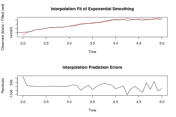
op <- par(mfrow=c(2,1))
plot(fit,ylab='Observed (black) / Fitted (red)',main='Interpolation Fit of Exponential Smoothing')
plot(myresid,ylab='Residuals',main='Interpolation Prediction Errors')
par(op)
dev.off()
bitmap(file='test2.png')
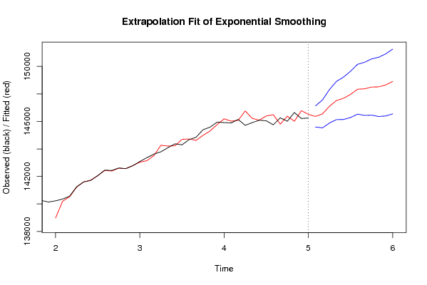
p <- predict(fit, par1, prediction.interval=TRUE)
np <- length(p[,1])
plot(fit,p,ylab='Observed (black) / Fitted (red)',main='Extrapolation Fit of Exponential Smoothing')
dev.off()
bitmap(file='test3.png')
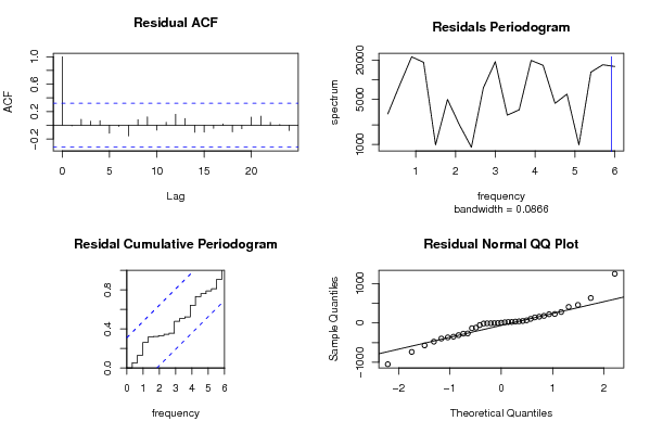
op <- par(mfrow = c(2,2))
acf(as.numeric(myresid),lag.max = nx/2,main='Residual ACF')
spectrum(myresid,main='Residals Periodogram')
cpgram(myresid,main='Residal Cumulative Periodogram')
qqnorm(myresid,main='Residual Normal QQ Plot')
qqline(myresid)
par(op)
dev.off()
load(file='createtable')
a<-table.start()
a<-table.row.start(a)
a<-table.element(a,'Estimated Parameters of Exponential Smoothing',2,TRUE)
a<-table.row.end(a)
a<-table.row.start(a)
a<-table.element(a,'Parameter',header=TRUE)
a<-table.element(a,'Value',header=TRUE)
a<-table.row.end(a)
a<-table.row.start(a)
a<-table.element(a,'alpha',header=TRUE)
a<-table.element(a,fit$alpha)
a<-table.row.end(a)
a<-table.row.start(a)
a<-table.element(a,'beta',header=TRUE)
a<-table.element(a,fit$beta)
a<-table.row.end(a)
a<-table.row.start(a)
a<-table.element(a,'gamma',header=TRUE)
a<-table.element(a,fit$gamma)
a<-table.row.end(a)
a<-table.end(a)
table.save(a,file='mytable.tab')
a<-table.start()
a<-table.row.start(a)
a<-table.element(a,'Interpolation Forecasts of Exponential Smoothing',4,TRUE)
a<-table.row.end(a)
a<-table.row.start(a)
a<-table.element(a,'t',header=TRUE)
a<-table.element(a,'Observed',header=TRUE)
a<-table.element(a,'Fitted',header=TRUE)
a<-table.element(a,'Residuals',header=TRUE)
a<-table.row.end(a)
for (i in 1:nxmK) {
a<-table.row.start(a)
a<-table.element(a,i+K,header=TRUE)
a<-table.element(a,x[i+K])
a<-table.element(a,fit$fitted[i,'xhat'])
a<-table.element(a,myresid[i])
a<-table.row.end(a)
}
a<-table.end(a)
table.save(a,file='mytable1.tab')
a<-table.start()
a<-table.row.start(a)
a<-table.element(a,'Extrapolation Forecasts of Exponential Smoothing',4,TRUE)
a<-table.row.end(a)
a<-table.row.start(a)
a<-table.element(a,'t',header=TRUE)
a<-table.element(a,'Forecast',header=TRUE)
a<-table.element(a,'95% Lower Bound',header=TRUE)
a<-table.element(a,'95% Upper Bound',header=TRUE)
a<-table.row.end(a)
for (i in 1:np) {
a<-table.row.start(a)
a<-table.element(a,nx+i,header=TRUE)
a<-table.element(a,p[i,'fit'])
a<-table.element(a,p[i,'lwr'])
a<-table.element(a,p[i,'upr'])
a<-table.row.end(a)
}
a<-table.end(a)
table.save(a,file='mytable2.tab')